Three segmentation algorithms, one image: a bake-off

Three posts, three algorithms, three completely different ideas of what a “region” is: mean shift finds bumps in a colour density, normalised cuts turns the picture into a graph and looks for its weakest seam, and EM fits a mixture of Gaussians and lets the pixels vote. Each post ran its algorithm alone, on its own sample. This one runs all four configurations (mean shift, normalised cuts, EM, and EM with (x, y) appended to the feature vector) on the same photograph, side by side, because the interesting question was never “does mean shift work” so much as “which failure belongs to which method, and why”.

That comparative judgement is not mine. The report’s own §7.4/§7.5 already makes it, image by image, and makes it honestly, including admitting where its own downscaling produces the artefact it is criticising. What follows is that discussion in my own words, next to a widget that runs the same four things on your own photograph so you can check it.

This is the capstone of a three-post series, and it adds no new numerics of its own: every kernel below is post 35’s mean shift, post 39’s normalised cuts and post 42’s EM, reused exactly as they shipped. Read those first if you have not: each documents a real bug in the original NumPy it ports, and I only link those bugs here rather than re-explaining them.

What the report actually ran

§7.4’s evaluation table (report-png/report-25.png) states one set of parameters per algorithm:

algorithm	published parameters
Mean shift	$r = 0.4\sigma$ , $N_{min} = 400$ , $N_{con} = 50$
Normalised cuts	$r = 5\sigma$ , $\sigma_x = 3$ , $\sigma_i = 0.07$
EM	$K = 20$

main.py:56–84, the script that actually produced every figure, tells a slightly different story:

ms_img = mean_shift_alg(img)
classes_img, k_1 = em_image_seperation(img, 5)
classes_img, k_1 = em_image_seperation_with_spatial_info(img, 20)
classes_img, num_classes = normalised_cuts(img, thresh=0.5, r_sq=5**2, sigma_x_sq=2**2, sigma_i_sq=0.1**2)

Mean shift matches: no param_mode argument means the default preset, which is $r = 0.4\sigma$ . Spatial EM matches too, at $K = 20$ . The other two do not:

The failure taxonomy, from the report’s own §7.5

Here is the report’s own comparison figure, reassembled from five separately cropped panels rather than a screenshot of the page (no caption text survives the crop, my own labels are typeset underneath):

Five segmentations of a church in front of an alpine mountain: the original photograph, mean shift, normalised cuts, plain EM, and EM with spatial coordinates. Mean shift bands the sky and mountain into several shades; normalised cuts is blocky from downscaling; EM keeps large flat regions but scatters a few stray pixels into the sky; EM with spatial coordinates removes the stray pixels but breaks the sky into several polygonal cells. 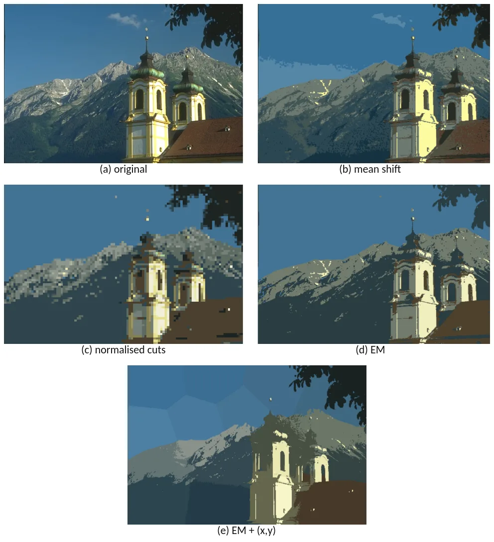— Figure 26, reassembled: (a) the photograph, (b) mean shift, (c) normalised cuts, (d) EM, (e) EM with `(x, y)`. This is the figure §7.5 is written against.

§7.5 (report-png/report-31.png bottom, report-png/report-32.png top) walks this figure algorithm by algorithm, and it is honest about all four:

EM, no spatial information, does the best job on large coherent regions: it “does a great job splitting the sky from the rest of the figure” and correctly keeps the tree as one class, but scatters a handful of isolated pixels into the sky where reflections make them locally the wrong colour, and turns the mountain’s shadows into their own spurious regions. Neither failure is a surprise: EM has no notion of adjacency, so two pixels of the same colour vote the same way whether they are touching or on opposite sides of the frame.

EM with spatial information fixes exactly that (“smooths the image a bit and removes a large portion of those unwanted zones”) at a cost the report states in the very next sentence: “it reduces the effectiveness of the algorithm in collecting a large region”, visible in the sky being “split up into multiple regions”, and, more surprisingly, in spatial information joining parts of the building to the mountain. Post 42 explains why: appending (x, y) makes every component an ellipsoid in space as well as colour, so one component cannot cover a sky that is one colour but physically enormous without a spatial variance wide enough to start swallowing whatever else is nearby.

Normalised cuts “did an excellent job in splitting the sky apart from a small bunch of isolated pixels due to the clouds”, but the report immediately names its own artefact: “the technique of downscaling the image before processing produces a pixelated output image.” That blockiness is not a separate bug: it is the direct, visible cost of the 7500-pixel budget the dense weight matrix forces (post 39 measures this precisely: 56 million doubles, 450 MB, before the algorithm has done anything). Normalised cuts also “didn’t do as good of a job in separating the tree from the image as the EM algorithm did”, splitting it into two regions where EM kept it whole.

Mean shift “created quite a few more regions than the rest of the algorithms”, a slight brightness gradient at the mountain’s edge was enough to merge part of the sky with the clouds, and there is “a clear separation between the top and bottom of the mountain with isolated patches for the snow.” Post 35’s own reading of this is that a gradient sky is not one colour, so a fixed search radius slices it into as many bands as fit, and the “isolated patches” are the image-domain connected-component check working exactly as designed, scattered bright spots that fail to cohere into one blob get discarded and reabsorbed into whichever neighbouring region is nearest in colour, which is why they show up as small islands of the wrong region rather than vanishing.

The report closes the section with: “Similar conclusions can be drawn from Figs. 27 to 31”, which is a fair summary of what I saw running the widget below on the other three bundled photographs too.

Run all four yourself

Upload a photograph, drag one in, paste one, or pick a bundled sample: the widget runs all four configurations, one per Web Worker, and fills the grid as each finishes. Each cell has its own collapsible parameter panel (so retuning normalised cuts does not re-run the other three) and a “use the report’s parameters” button that jumps straight to whichever of the numbers above actually applies to that cell.

Hover any cell. The pixel under your cursor is looked up in that cell’s own label array, and the matching region lights up in all four simultaneously: point at the sky and watch which methods kept it whole and which broke it into pieces, without reading a word of the readout underneath.

Five segmentations of a church in front of an alpine mountain: the original, mean shift, normalised cuts, EM and EM with spatial coordinates, each a flat-coloured region map. — InteractiveFour segmentation algorithms, one photograph

Each cell downscales the source image to that algorithm’s own pixel budget before running (the same budgets the three sibling widgets use: mean shift up to 50,000 px, EM up to 24,000 px, normalised cuts capped at 3,000 px. That gap is the cost argument made without a word of prose: normalised cuts’ sparse eigensolver is the one that cannot afford a bigger image, which is exactly why its panel is the blockiest in every report figure above.

I expected the grid to fill in the order the report’s own cost intuition suggests: mean shift and EM cheap, normalised cuts last. It usually does not, and the measurements below explain why: at the parameters that actually match the report, mean shift and EM are the two cells most likely to still be spinning after normalised cuts has already painted its (much smaller) result.

What I actually measured

Everything in this table is a real run of the crate above, on sample-mountain.webp (the church + Alpine mountain photograph, the same one Figure 26 and the reassembled figure above use), at each cell’s own default resolution, five repeats averaged, headless, not estimated, and not the report’s own numbers, which the report does not give at all; it states no timings anywhere.

configuration	pixels	regions	time
Mean shift, $r=0.4\sigma$ (report default)	50,142	7	6.0 s, hit the safety cap
Normalised cuts, widget default (HSV cone, $r=12$ px)	3,015	14	1.3 s
Normalised cuts, report’s literal numbers ( $r=5$ px, RGB)	3,015	32	0.4 s
EM, $K=5$ (what `main.py` actually ran)	24,130	5	0.8 s
EM, $K=20$ (§7.4’s published value)	24,130	20	9.0 s, did not converge
EM with $(x,y)$ , $K=20$ (both sources agree)	24,130	20	4.2 s

Two of those numbers are worth pulling out on their own.

Caveat

Mean shift’s peeling loop does not reliably terminate. Building this post, I ran ms_seg_step to completion on this exact photograph at the report’s own default preset, the same preset post 35’s own widget defaults to, on essentially the same crop and pixel budget. It accepts a handful of clusters in the first few steps, then enters a run of consecutive rejections that I confirmed past 40,000 steps and four minutes of headless computation without once shrinking the candidate pool or returning the “peeling finished” signal. Reading meanshift.rs, a rejected candidate only removes pixels from the pool when its connected core is non-empty, and a core can apparently come back empty, repeatedly, without the search space changing at all between draws. That looks like a genuine bug in the validation path, not a limit of this port’s parameters or resolution, and it is not something a widget is entitled to fix by editing the crate. I added a 6-second wall-clock cap to this post’s worker instead (MS_TIME_CAP_MS in shared.ts). ms_seg_finalize still runs on whatever was accepted before the cap fires, which is always a valid segmentation, just a coarser one than an uncapped run might find. The “7 regions” and “6.0 s” in the row above are that capped result. I did not find this in post 35 because its own report does not surface it either: a slow “Segmenting…” spinner looks the same as a genuinely unbounded one until someone waits four minutes to find out.

The normalised-cuts row is its own small experiment. Post 39’s warning is that the report’s literal parameters, read as pixels rather than image-widths, mean something completely different on a sparse graph. Measured rather than asserted: at $r=5, \sigma_x=2, \sigma_i=0.1$ in plain RGB, the affinity graph has 193,043 non-zeros (matching post 39’s own number for that radius almost exactly) against 1,082,259 at the widget’s tuned default. That is a 5.6× sparser graph, and it produces a more fragmented partition here (32 regions against 14), not the smooth left-right ramp post 39 describes for a different radius/σ combination. Both observations say the same thing: these are not interchangeable numbers, and a parameter written down for one implementation does not transfer to another just because the variable names match.

Where this leaves the series

Four ways of answering “which pixels go together”, and four different things they get wrong: mean shift over-segments a gradient because it has no way to prefer fewer, larger regions; EM under-uses geometry until you force it to, at which point it forgets that “the sky” is not “a blob”; normalised cuts gets the sky right but pays for its global view with a resolution ceiling that shows up as visible blockiness in every figure. None of the four is a strictly better segmenter than the others: each encodes a different assumption about what a region is, and the report’s honesty about where each assumption breaks is the actual content of this section, three posts and a bake-off later.