Blog · Segmentation ·
Fitting Gaussians to pixels: EM, and what happens when you tell it where the pixels are
Model an image's colours as a mixture of K Gaussians and fit it by Expectation-Maximisation. Then append each pixel's (x, y) to its colour vector and watch the segments become compact, and the sky fall apart.
- Interactive
- segmentation
- expectation-maximisation
- gaussian-mixture-model
- clustering
- wasm
A pixel does not belong to a region. It belongs 0.7 to one region, 0.3 to another, and 0.0000001 to the rest, and if you are willing to say that out loud, a whole family of clustering algorithms opens up that hard assignment cannot reach.
That is the idea behind fitting a Gaussian mixture model to an image. Each region of the picture is a blob of colours in some feature space; a blob is a multivariate normal distribution; the image as a whole is a weighted sum of of them. Fit the mixture and the segmentation falls out as a by-product: every pixel’s label is just which component claims most of it.
The fitting is done by Expectation-Maximisation, which is two lines of intuition and about twelve of NumPy: work out how much each blob is responsible for each pixel (the E step), then move every blob to the weighted mean of the pixels that claimed it (the M step), and repeat until nothing moves.
The reason I still find this experiment worth writing up ten months later is not the algorithm. It is a one-line change at the end. Append each pixel’s coordinates to its colour vector, so the Gaussians live in 5-D instead of 3-D , and the segmentation goes from scattered colour classes to spatially compact blobs. It fixes exactly the thing you wanted fixed. It also breaks something you did not think to protect.
Two equations and a recipe
The report sets this up in half a page (§7.3, p. 24–25). Each component is a multivariate normal with its own mean, covariance and prior, so the probability of the -th feature vector under component is
and what we want to maximise is the log-likelihood of the whole feature matrix under the mixture:
Differentiating 7.7 with respect to , and and setting each derivative to zero gives the update rules: Eqs 7.8 to 7.10, with the responsibility from Bayes’ rule in 7.11 and the normaliser in 7.12:
And the recipe, as the report lists it:
- Initialise random distributions.
- Calculate by Eq 7.11: the E step.
- Maximise the likelihood with respect to , and using Eqs 7.8–7.10: the M step.
- Repeat until the likelihood of Eq 7.7 has converged.
Notice what actually is. Eq 7.12 says it is the total responsibility component holds across the whole image: the effective number of pixels that belong to it. So 7.8 is a weighted average, 7.9 is a weighted covariance about that average, and 7.10 is “what fraction of the image is you”. Three equations, one idea: every pixel votes, with fractional votes, and each blob becomes the shape of its voters.
Watch it run
The widget below is that loop, one half-step at a time. On the left, the image’s pixels plotted in the – plane with the components drawn as ellipses at one standard deviation, each tinted with the mean colour of the pixels currently claiming it. On the right, the segmentation: every pixel painted with its class’s mean colour, which is exactly how the report renders its figures. Underneath, the log-likelihood of Eq 7.7 traced per iteration.
Step E and Step M are separate buttons because the two halves look completely different. E redistributes the votes: the point cloud recolours, but nothing moves. M snaps the ellipses onto their new means and reshapes them to their new covariances. Play alternates the two at a rate you can watch.
Then flip include (x, y) and run it again.
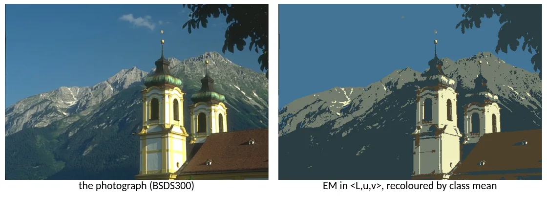
With JavaScript on, this becomes an interactive fit: a scatter of the image’s pixels in the u–v plane with the mixture components drawn as ellipses, a live segmentation, and separate Step E / Step M controls. You can drop in your own photograph and download the result.
Three things worth doing with it:
- Press Reseed a few times at K = 5. The initial means are a uniform draw from the data’s bounding box, so different seeds walk into different local optima and give genuinely different segmentations. EM does not have an answer; it has an answer per starting point. (Reset, next to it, rewinds to iteration zero with the same draw, so you can watch one fit twice.)
- Watch the log-likelihood. It climbs steeply for three or four iterations and then crawls. That is the whole reason the stopping rule is a relative test rather than a fixed number of iterations.
- Turn on (x, y) and look at the sky. Read on.
The code, which is the equations
Algorithms/ExpectationMaximiser.py is 95 lines and maps onto those equations almost
symbol for symbol. A component is a class holding one scipy normal and its prior
(lines 7–25):
class Distribution:
    def __init__(self, data, k):
        data_dim = len(data[0])
        mean = np.random.uniform(np.min(data, axis=0), np.max(data, axis=0))
        var = np.max(data, axis=0) - np.min(data, axis=0)
        self.dist = multivariate_normal(mean, np.eye(data_dim)*var)
        self.prior = 1.0/k

    def calc_expectation(self, data):
        return self.dist.pdf(data)*self.prior

    def maximise_dist(self, data, weights, expectations):
        self.dist.mean = np.sum((data.T*weights).T, axis=0)
        dist_from_mean = data-self.dist.mean
        self.dist.cov = np.dot(dist_from_mean.T*weights, dist_from_mean)
        self.prior = np.average(expectations)
calc_expectation is the numerator of Eq 7.11. maximise_dist is Eqs 7.8, 7.9 and 7.10
in that order: weights arrives already divided by , so the two np.sums are
the weighted mean and the weighted covariance, and np.average(expectations) is
, since the average of a component’s responsibilities over all pixels is its
share of the image.
The initialisation is worth staring at. var is the range of each dimension
(max - min), and it is handed straight to multivariate_normal as a variance. For
8-bit Luv that is a variance of up to 255 in each channel, i.e. a standard deviation of
about 16 colour levels, which makes the initial blobs enormous and heavily overlapping.
That is not a bug so much as a shrug, but it is why the first iteration moves so far.
The loop itself (lines 28–54):
def perform_em(X, k, thresh=1e-12, m=1000000):
    distributions = [Distribution(X, k) for i in range(k)]

    expectations = np.zeros((len(distributions), len(X)))
    for i, d in enumerate(distributions):
        expectations[i] = d.calc_expectation(X)
    scale_exp = np.sum(expectations, axis=0)
    log_likelihood = np.sum(np.log(scale_exp))

    for j in range(m):

        expectations /= scale_exp
        weights = (expectations.T/np.sum(expectations, axis=1)).T

        for i, d in enumerate(distributions):
            d.maximise_dist(X, weights[i], expectations[i])
            expectations[i] = d.calc_expectation(X)

        scale_exp = np.sum(expectations, axis=0)
        log_likelihood_curr = np.sum(np.log(scale_exp))
        print(log_likelihood/log_likelihood_curr)

        if log_likelihood/log_likelihood_curr < 1.0+thresh:
            break
        log_likelihood = log_likelihood_curr
expectations /= scale_exp is Eq 7.11, all rows at once. The line after it divides
each component’s row by its own total (that total is from Eq 7.12), so
weights[i] is the pre-normalised weighting Eqs 7.8 and 7.9 want. Twelve lines, six
equations, no scaffolding. I still like it.
The convergence test is a ratio
The stopping rule is the one part I would write differently now:
if log_likelihood/log_likelihood_curr < 1.0+thresh:
    break
That is a ratio of successive log-likelihoods, not a difference, and it has three distinct problems.
It is scale-dependent. Double the number of pixels and the log-likelihood roughly
doubles, so the same thresh = 1e-12 becomes twice as strict for the same per-pixel
improvement. A tolerance that means one thing on a 481 × 321 photograph means another on a
thumbnail.
It is sign-unsafe. The test only behaves like a stopping rule while the log-likelihood
is negative. These are continuous densities, so a fit on tightly clustered data can easily
push the log-likelihood positive, at which point an improving fit has
old / new less than 1 and the loop breaks on its first iteration.
And it is one-sided: < 1.0 + thresh fires on any ratio below one, which is to say on
any step where the log-likelihood went down at all. I measured this in the port. Over 20
runs of the church photograph across two feature spaces, two values of and five seeds,
18 stopped because the log-likelihood dipped rather than because it plateaued, mostly
by a relative , which is genuinely the noise floor of a converged fit, but twice
by around , which is an early stop with real iterations left in it. Some of
that wobble is mine: I keep the responsibility matrix in f32 and add a small ridge to every
covariance, and both put a floor under how flat the curve can get. But the mechanism does
not depend on my choices: a one-sided test cannot distinguish “converged” from “the first
step that did not improve”.
An absolute test on the per-pixel change, (curr - prev) / N < ε with a patience of two or
three iterations, would have been scale-free, sign-safe and two-sided. The widget reports
the actual ratio next to the log-likelihood so you can watch it squeeze towards 1 and then
tip under it.
Where the segmentation actually comes from
Two functions, differing by one line (57–74):
def em_image_seperation(img, k, thresh=1e-7, max_it=1000000):
    img_data = cv2.cvtColor(img, cv2.COLOR_BGR2Luv).reshape((-1, img.shape[-1]))
    expectations = perform_em(img_data, k)

    img_out = np.zeros(img.shape[:-1])
    img_out.flat[:] = np.argmax(expectations, axis=0)
    return img_out, k


def em_image_seperation_with_spatial_info(img, k, thresh=1e-7, max_it=1000000):
    img_data = cv2.cvtColor(img, cv2.COLOR_BGR2Luv).reshape((-1, img.shape[-1]))
    ind = np.indices(img.shape[:2]).reshape((2, -1)).T
    img_data = np.hstack((img_data, ind))
    expectations = perform_em(img_data, k)

    img_out = np.zeros(img.shape[:-1])
    img_out.flat[:] = np.argmax(expectations, axis=0)
    return img_out, k
That np.hstack is the whole experiment. The report puts it in one sentence: “both the
and the feature-spaces were tested.”
The colour space matters more than it looks. cv2.COLOR_BGR2Luv on an 8-bit image does
not just convert to CIE L*u*v*, it also packs the result back into bytes, with
, and
. All three channels end up on 0…255. That is what makes
appending a raw pixel coordinate to the vector a sensible thing to do at all: a BSDS300
photograph is 481 × 321, so and land on a comparable scale to the colour channels
without anybody having to choose a weight. Nobody wrote that down; it is a coincidence of
two byte ranges, and it is doing a lot of work.
Finally, the rendering (lines 77–83):
def get_color_image_from_classes(k, classes_img, img):
    out_img = np.zeros(img.shape)
    for class_id in range(k):
        ind_c = np.where(classes_img == class_id)
        class_avg_int = np.average(img[ind_c], axis=0)
        out_img[ind_c] = class_avg_int
    return out_img
Every pixel is painted with the mean of the original colours of its class, not with the Gaussian’s mean, and not with a palette. That is why the figures look like posterised paintings rather than a false-colour map, and it is a genuinely good choice: a segmentation you can compare with the photograph by eye.
What I changed, porting it to Rust
The widget above runs the same algorithm compiled to WebAssembly, because the point of it
is smooth per-iteration animation, and a 5-D fit over 24 000 pixels at is half a
million Gaussian evaluations an iteration, about 40 ms of work, which is fine at a
half-step every fifth of a second and hopeless in a for loop over pixels in JavaScript.
Two things in the port are deliberately not what the Python does, and both are numerical.
The E step accumulates in log space. scipy’s pdf returns a density, and in this
feature space the densities get very small. I instrumented a converged fit of the church
photograph and looked at the Mahalanobis distance from each pixel to each component: at
in the largest reaches about 124 000. is not a small
number in a float64; it is exactly zero. So a large share of the Python’s expectations
matrix is hard zeros, in all eight configurations I probed, across both feature spaces,
both values of and two seeds each.
The mixture sum survives that: some component is always near enough, and the worst
per-pixel I measured was about , so np.log(scale_exp) stays finite and the
log-likelihood is fine. The line that is not fine is the next one:
weights = (expectations.T/np.sum(expectations, axis=1)).TThat divides each component’s row by its own total, which is from Eq 7.12. A
component that has been outvoted at every single pixel, because every one of its densities
underflowed, has a total of exactly zero, and is nan. The nan goes into that
component’s mean and covariance, out through its calc_expectation, into scale_exp, and
from there into every other component’s responsibilities on the next pass. One starved
blob and the whole fit is silently gone.
Working in logs removes the first problem outright: each component contributes , and the normalisation is a log-sum-exp with the row maximum pulled out first, so a term at contributes nothing without destroying anything.
pub fn log_sum_exp(a: &[f64]) -> f64 {
    let mut m = f64::NEG_INFINITY;
    for &v in a {
        if v > m { m = v; }
    }
    if !m.is_finite() { return m; }
    let mut s = 0.0;
    for &v in a { s += (v - m).exp(); }
    m + s.ln()
}
It also makes the second problem visible rather than silent: a component whose total responsibility falls below is detected and re-drawn from the data instead of being divided by. There is a test for exactly the underflowing case, on points 400 units apart in a space where every density rounds to zero, the responsibilities still come out summing to one.
Σ is kept as its Cholesky factor. multivariate_normal re-decomposes the covariance on
every call; storing instead gives the log-determinant as
and the Mahalanobis distance as
by forward substitution: no general matrix inverse anywhere, and the factorisation is
the positive-definiteness check, so a component whose covariance has collapsed announces
itself instead of returning NaN.
One more departure, which is an honest patch rather than an improvement: I add a ridge of
of each dimension’s data variance to every covariance diagonal. Luv here is
quantised to bytes, so a component that lands on a run of identical pixels collapses to a
zero-volume Gaussian with unbounded likelihood, the classic EM singularity. The NumPy has
no guard at all; scipy simply raises. A starved component (one nobody voted for) is
likewise re-drawn rather than left to produce NaN. Both make the widget survive parameter
choices the batch script never had to.
The results, and the honest half of them
Here is the comparison the report drew, on the two images where it reads most clearly. Panel (d) in each figure is plain EM in ; panel (e) is the same algorithm in .
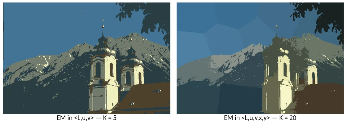
The report’s Figure 26, panels (d) and (e), re-cropped and relabelled. Spatial information removes the isolated stray pixels and joins parts of the building to the mountain, and chops the sky into Voronoi-like cells.
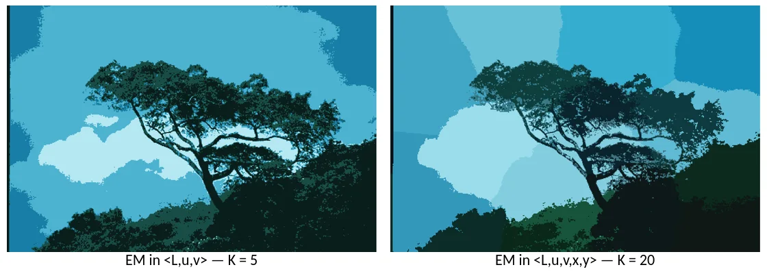
Figure 30, panels (d) and (e). The same trade in a picture with a much simpler colour histogram: the cloud gets cleaner edges, the sky stops being one thing.
The report’s own verdict, in §7.5, is refreshingly unsold on its own experiment. On the plain fit it is positive: EM “does a great job splitting the sky from the rest of the figure” and “a really good job of associating all the pixels belonging to the tree together”. It even explains the mountain being split into three, rather than calling it an error: the mountain really does go trees, then rock, then patches of ice, and EM found all three. The failure it names is small and specific: a handful of isolated pixels assigned to the sky, which it attributes to “the fact that no spatial information is given to this algorithm and those pixels are close in colour to the sky due to reflections”.
And then the fix, and its cost, in one breath: giving EM spatial information “smooths the image a bit and removes a large portion of those unwanted zones. However, it reduces the effectiveness of the algorithm in collecting a large region. This can be seen in the sky, which is now split up into multiple regions.”
Which is exactly right, and exactly what you would predict if you thought about it for a minute. A Gaussian in is an ellipsoid in space as well as in colour. A region that is one colour but physically enormous, a sky, cannot be covered by one such ellipsoid without a spatial variance so large that it starts swallowing the mountain too. So the fit does the only thing available to it and tiles the sky with several components, which is why panel (e) looks like a Voronoi diagram wherever the picture is flat. The very same mechanism that glues stray pixels to their neighbours forbids any region from being much bigger than a blob.
So I ran the comparison the report meant to run. Same photograph (the crop of Figure 26’s
panel (a) that the widget bundles), my Rust port, 190 × 127 = 24 130 pixels, the same
1e-12 ratio test, three random seeds averaged, both feature spaces at the same :
| measurement | K = 5, ⟨L,u,v⟩ | K = 5, ⟨L,u,v,x,y⟩ | K = 20, ⟨L,u,v⟩ | K = 20, ⟨L,u,v,x,y⟩ |
|---|---|---|---|---|
| connected regions of ≥ 20 px | 29.7 | 21.7 | 85.7 | 51.3 |
| specks of fewer than 4 px | 227 | 180 | 1113 | 369 |
| distinct classes across the sky | 2.0 | 3.7 | 4.0 | 6.0 |
Both halves of the report’s verdict survive the correction. Adding at matched roughly cuts the number of stray sub-4-pixel specks by a fifth at K = 5 and by two thirds at K = 20, and cuts the number of separate regions by a quarter and by two fifths respectively, and that is the smoothing the report describes. It simultaneously spends more components on the sky, 2.0 → 3.7 and 4.0 → 6.0, which is the fragmentation it complains about. The effect is real; the report’s own figure just overstates it by changing two things at once.
Where I would take it next
The report ends its own paragraph with a suggestion I have never got round to trying, and it is the right one:
It may be possible to rectify this by encoding the spatial information in a different way such as using polar co-ordinates.
Think about what that would buy you. Cartesian makes “compact” mean “a small elliptical patch”, which is a poor description of a sky, a horizon or a road. Polar coordinates about the image centre would make a component’s spatial extent an annulus or a wedge, which is a much better description of the way a photograph is usually composed: sky at the top spanning the full width, ground at the bottom, subject in the middle. A single Gaussian in can be “everything far from the centre, at any angle” in a way that no Gaussian in can be.
That is only one of the encodings worth trying. Any monotone squashing of the coordinates, say of the distance from the centre, would cap how much the spatial term can dominate once a component is already large, which is the actual failure here: the spatial penalty keeps growing linearly while the colour term saturates. So does simply scaling the columns down, which is the one-parameter version of the whole question and which nobody in this report tuned, because the byte packing chose it for us by accident.
The deeper point is that appending coordinates to a feature vector is not a neutral act. It does not “add spatial information” to the model; it asserts that regions are ellipsoidal in space, which is a strong prior and, for photographs, usually a wrong one. Every improvement it makes and every one it breaks follows from that single assumption. It was worth doing precisely because it is so cheap to try, and worth writing up because the result was ambivalent rather than clean.
The other two algorithms in this section (mean shift, which does not make you pick at all, and normalised cuts, which turns segmentation into an eigenvalue problem) take completely different routes to the same “which pixels go together” question. They get their own posts.