Blog · Segmentation ·
Normalised cuts: segmentation as an eigenvalue problem
Every pixel is a node, every edge weight says how alike two pixels are, and segmentation becomes graph partitioning. Minimum cut gets it wrong; Shi and Malik's fix turns the whole thing into an eigenvector you can look at.
- Interactive
- segmentation
- graph-partitioning
- eigenvectors
- lanczos
- wasm
Of the three segmentation algorithms I wrote for this section of the report, normalised cuts is the one I still think about. The other two are clustering with extra steps. This one takes a picture, turns it into a graph, and then produces (as an eigenvector of a matrix) something that is unmistakably a picture of the scene’s structure. You can look at a linear-algebra object and see a mountain in it.
That is the whole reason this post has a widget. The middle panel below is the second-smallest eigenvector of a 3015 × 3015 generalised eigenvalue problem, drawn as a heatmap over the pixels it came from. Nobody told it where the sky was.
An image is a graph
Take every pixel to be a node. Join pairs of pixels with an edge whose weight says how alike and how close they are. Segmentation is now graph partitioning: split the node set into two disjoint halves and and pay for every edge you sever.
The obvious objective is to sever as little as possible. That total is the cut, and Eq 7.1 of the report is the standard definition:
Minimum cut is a solved problem: it is max-flow, it is polynomial, it is in every textbook. It is also, for this purpose, useless, and the reason is worth being concrete about.
Minimum cut always lops off a corner
Here is a graph with seven nodes. Two triangles of three, every internal edge weight 1, joined to each other by a single bridge of weight 0.2. Hanging off one of them is a lonely node , attached by an edge of weight 0.1.
Two candidate partitions. Minimum cut prefers the left one, which is the wrong answer.
There are two sensible ways to cut this. Sever the bridge and you get two clusters of three, at a cost of 0.2. Sever the outlier’s one edge and you get a partition of six against one, at a cost of 0.1.
Minimum cut takes the cheaper number and returns the useless partition. The report puts it in one sentence, and it is exactly right:
This approach tends to cut off small regions with few connections as these have the smallest impact on the weight.
There is nothing pathological about that example. It is the generic behaviour: a lonely node has few edges, so severing all of them is cheap, so it is always the first thing minimum cut reaches for. On a photograph, the lonely node is the pixel in the corner.
Normalise by how well-connected each side is
Shi and Malik’s fix is to divide the cut by the total connection each side has to the whole graph, so a partition is only cheap if both sides were substantial to begin with. Eqs 7.2 and 7.3:
is just the sum of the degrees of ‘s nodes. Run the two candidate partitions through it. The degrees are , , , , and , so the whole graph has .
Lop off the outlier. , , :
Sever the bridge. , , :
The outlier’s cut was half the price and its Ncut is sixteen times worse. That first
term is the whole trick: severing everything a node owns makes
, and the ratio pins at 1 no matter how small the
weights are. You cannot buy your way out of it by being lonely. (Both of those numbers are
a unit test in the port: ncut_of_a_known_partition_matches_hand_arithmetic.)
The weights
Eq 7.4 is a product of two Gaussians: one on distance in feature space, one on distance in the image, hard-zeroed past a radius .
is the pixel’s feature vector, its position. The denominators are written as
and in the report but the code passes their squares
(sigma_i_sq=0.07**2, sigma_x_sq=3**2), so read them as throughout.
That otherwise 0 is the single most important line in the algorithm, and not for the
reason it looks like. It is what makes sparse, and sparsity is the only
reason any of this is computable. More on that below, because the implementation in the
repo manages to switch it off by accident.
Here is calculate_weights in full, from Algorithms/NormalisedCuts.py:49–58:
def calculate_weights(img_flat, img_ind, r_sq=5**2, sigma_x_sq=3**2, sigma_i_sq=0.07**2):

    square_dist = np.sum(np.square((img_ind[:, None] - img_ind) / np.max(img_ind)), axis=2)
    ind_hold = np.where(square_dist < r_sq)
    weights = np.zeros(square_dist.shape)
    weights[ind_hold] = np.exp(-square_dist[ind_hold] / sigma_x_sq)

    square_dist = np.sum(np.square(img_flat[ind_hold[0]] - img_flat[ind_hold[1]]), axis=1)
    weights[ind_hold] *= np.exp(-square_dist / sigma_i_sq)
    return weights
The feature space, and the file that got it right
The report notes what the original paper uses:
The feature-space used in the original paper is , where is from the HSV colour space.
That is HSV mapped onto a cone. It exists because hue is an angle, so the raw difference between and is enormous while the colours are identical, and because hue is meaningless for a grey pixel, where any hue at all should collapse to the same point. Multiplying by does both: near-grey pixels () and near-black pixels () land on the cone’s axis regardless of hue.
NormalisedCuts.py does not do this. It min-max normalises the whole image to and
feeds raw BGR straight in (NormalisedCuts.py:81–84). What does implement the cone is
the file next to it: NormalisedCuts - Copy (2).py:85–88:
img_flat_features = cv2.cvtColor((img/255).astype(np.float32), cv2.COLOR_BGR2HSV_FULL).reshape((-1, scaled_img.shape[-1]))
s = img_flat_features[:, 1].copy()
img_flat_features[:, 1] = img_flat_features[:, 2]*s*np.sin(img_flat_features[:, 0] * np.pi / 180)
img_flat_features[:, 0] = img_flat_features[:, 2]*s*np.cos(img_flat_features[:, 0] * np.pi / 180)
The same file also computes the weights properly: accumulating both exponents in the log
domain and calling exp once at the end, rather than multiplying two separate exp
results (- Copy (2).py:54–58). Both of these are improvements. The variant that got the
maths right was the one I left as a scratch file and never wired into main.py, which is
about as neat a summary of that week as I can offer.
The relaxation, and why it is an eigenvalue problem
This is the part that makes the algorithm beautiful. Minimising Eq 7.2 over all partitions is NP-hard. But write the partition as a vector that assigns each pixel to a class, and Ncut turns out to be a Rayleigh quotient:
where holds the weights and is diagonal with , the degree of pixel . Constrained to the two discrete values that mean “in ” and “in ”, that minimisation is the original hard problem. Relax it: let take any real value, and the minimiser of a Rayleigh quotient is an eigenvector. Eq 7.5:
is the graph Laplacian, so is always a solution with (the partition that puts everything on one side, which is no partition at all). The one you want is the second smallest: the smallest non-trivial direction in which the graph can be pulled apart. The report is characteristically brisk about it:
This is done efficiently using the Lanczos method as the matrix is sparse and a high precision of the eigenvectors is not required. Furthermore, only the smallest few eigenvalues are needed.
Turning a real vector back into a partition
is real-valued, so you still have to choose where to cut it. The algorithm’s
answer is not clever and does not need to be: sample twenty evenly-spaced thresholds
across the range of , score each with Eq 7.2, and take the best
(NormalisedCuts.py:23–43).
That is the slider in the widget. Drag it and the third panel repartitions live while a marker moves along the plot of Ncut against threshold; press Snap to best to jump to the minimum of the twenty points the algorithm itself would have evaluated. It is worth hunting for the minimum by hand first. The curve has a characteristic shape: a steep wall on the left where the partition is one lonely fragment and the first term of Eq 7.2 is pinned near 1, then a long shallow basin across every sensible split. It is the wall, not the basin, that Ncut bought you.
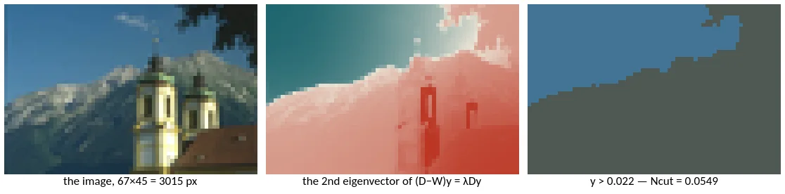
With JavaScript on, this becomes a live solver: sliders for σ_I, σ_X, the connection radius and the pixel budget, a threshold you can drag along the Ncut curve, an eigenvector selector, and a Recurse button that draws the tree of regions. Upload or paste your own photograph and download the segmentation.
Things worth doing in there:
- Watch the eigenvector, not the segmentation. Panel 2 is the point. The partition in panel 3 is just panel 2 with a threshold applied.
- Switch feature space. RGB is what
NormalisedCuts.pyuses; the HSV cone is Shi and Malik’s own; Luv is what the other two algorithms in the repo use. On the mountain, the cone separates sky from rock and the raw RGB does not. - Set σ_I to 0.07, σ_X to 3, r to 5 and the feature space to RGB. Those are the report’s own published parameters (§7.4) taken literally, in pixels. The second eigenvector’s Ncut curve then spans only 0.044 (under the 0.06 guard below), so the algorithm rejects it and moves to the third. See the next section for why that happens.
- Pull the pixel budget up and down and watch “solver ms” in the readout. That number is the whole story of this algorithm’s reputation.
The two guards
Algorithm 2 of the report (p. 24) is twenty lines. Transcribed:
procedure NORMALISED CUT(F, X, α)
    W ← weight values according to Eq 7.4
    d ← values according to Σⱼ w(i, j)
    D ← d · I
    i ← 2
    N_i ← number of eigenvalues produced
    repeat
        y ← the eigenvector belonging to the index i eigenvalue produced by
            Eq 7.5, in ascending order
        Ncut_min, Ncut_max ← the minimum and maximum Ncut values produced by
            different thresholds
        ind_A, ind_B ← the indices of partitions A and B which produce the
            minimum Ncut
        i ← i + 1
        if i ≥ N_i and Ncut_max − Ncut_min < 0.06 then
            return X, ∅
        end if
    until Ncut_max − Ncut_min ≥ 0.06
    if Ncut_min > α then
        return X, ∅
    end if
    return NORMALISED CUT(F[ind_A], X[ind_A], α), NORMALISED CUT(F[ind_B], X[ind_B], α)
end procedure
Two things in there are not in the paper, and both are the kind of thing you only add after watching an implementation misbehave.
The 0.06 spread test. If sweeping the threshold across an eigenvector barely changes the Ncut, that eigenvector is not telling you where to cut: every split it offers costs about the same, so the choice is arbitrary. Move to the next one.
The constant is less arbitrary than it looks. Ncut lives in , and there is a specific value that means no information at all: if every weight in the graph is equal, then for any partition of size out of , , and , so
exactly, for every . A completely uninformative graph gives a dead-flat curve pinned at
- The test is “how far is this curve from dead flat”, and 0.06 is the tolerance. That
identity is also a test in the port:
flat_guard_fires_when_every_pixel_is_the_same.
The test. If even the best threshold costs more than , stop cutting this region: it is not made of two things. This is the recursion’s only real stopping criterion, and it is what decides how many regions you end up with. On the mountain at the widget’s defaults, all thirteen leaf regions stop on this test and none on the other two.
The port: why this one needed Rust
Look again at what calculate_weights builds. square_dist is an dense
NumPy array. At the report’s own budget of 7500 pixels that is 56.25 million doubles,
450 MB, before you have started; the widget’s default of 3015 pixels would still be 9.09
million entries and 73 MB. And it is thrown away almost entirely, because past the radius
every entry is zero.
The port keeps the same matrix in compressed sparse row. At the widget’s default
radius of 12 pixels each row holds about 359 entries (1.08 million non-zeros, a few MB),
and at the report’s radius of 5 it is 64 a row, 193 043 non-zeros, which is 2% of the
dense matrix. The kernels are in wasm/crates/segment-wasm/src/ncut.rs; the widget only
owns the DOM.
Then there is no scipy.sparse.linalg.eigsh to call, so the eigensolver is hand-written.
The trick that makes it tractable is a change of variable. Substituting
turns the generalised problem into a standard
symmetric one,
and writing , the eigenvalues of are for an eigenvalue of . So the smallest eigenpairs of the problem we want are the largest of , and the largest end is the one Lanczos converges to fastest. The trivial becomes with , which is known in closed form, so it is projected out of every Lanczos vector rather than computed.
The other departure is deliberate and is the subject of the next section: and
are in pixels here, not in the units NormalisedCuts.py actually measures
them in.
The bug that makes the original work
Look at line 51 again:
square_dist = np.sum(np.square((img_ind[:, None] - img_ind) / np.max(img_ind)), axis=2)Pixel coordinates are divided by np.max(img_ind) (the largest index in the image, i.e.
the long side minus one). So distances are measured in image widths, and land in
. The radius test is then square_dist < 25, which is true for every pair
of pixels in the image. The otherwise 0 branch of Eq 7.4 never fires. is
dense (genuinely, all 56 million entries of it), which is exactly why the code allocates a
dense array and why 7500 pixels was the ceiling.
It gets better. With distances on and , the spatial factor
ranges from 1 to 0.85 across the entire frame. The spatial term is not a
locality constraint at all; it is a 15% tilt. What NormalisedCuts.py actually computes is
colour affinity between every pair of pixels in the image, with a whisper of position
on top.
And here is the thing: that is why it works. When I first ported this faithfully (radius in pixels, , ) the second eigenvector came out as a smooth left-to- right ramp on every image I tried, because a 67-pixel-wide lattice with strong local connections has, as its slowest mode, a gradient along its long axis. The colour structure could not compete. To get the report’s own pictures back I had to make the neighbourhood large () and the spatial falloff gentle within it (), so that the spatial term becomes a soft window rather than a lattice, which is a sparse approximation of the dense all-pairs graph the bug produced.
- Copy (2).py:51 drops the division and measures in pixels, with and
: the version whose radius genuinely bites, and the one whose parameters
transfer to a sparse implementation. Second time that scratch file has been the better one.
A couple more things I found rereading it
Recursion
One cut gives you two regions. Cut each of those the same way and stop when the
test fires, and you have the full segmentation: Algorithm 2’s last line, and
recursive_normalised_cuts (NormalisedCuts.py:61–69).
The Recurse button in the widget does this one region at a time so the tree draws itself as it grows, which is more informative than watching a frozen page for a second. On the mountain at the defaults it produces 25 nodes and 13 leaf regions in about a second and a half, every leaf stopping because its best Ncut exceeded . Click a node in the tree (or pick it from the dropdown) and that region is highlighted in the segmentation, with the reason it stopped printed underneath.
Two things are visible in the tree that are not visible in the segmented image. The first is that the cuts are strongly unbalanced: the root splits 2021 against 994, and the Ncut of a split climbs steadily with depth (0.056, then 0.074 and 0.234, then 0.085 and 0.324) until it crosses . The second is that the recursion has no idea the regions are supposed to be connected: a leaf can be two unrelated patches that happened to sit on the same side of a threshold. Mean shift, the algorithm before it in the report, validates every cluster against the image-domain connected components and throws away the ones that fail. Normalised cuts has no such check.
Why the output is blocky
Every panel (c) in the report’s comparison figures looks like this:
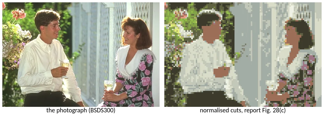
Figure 28 of the report, panels (a) and (c). The labels are mine. The blocks are not a rendering artefact: they are the pixels of the downscaled image, upscaled back with nearest-neighbour interpolation.
The report says why, flatly, in the paragraph after Algorithm 2:
The original normalised cut algorithm is slow on large images. Hence it was decided to scale large images down to smaller images containing no more than 7500 pixels. This was then put through the Normalised Cut algorithm. The resulting image containing various regions was then up-scaled using nearest neighbour interpolation.
and again in the discussion, §7.5:
The normalised cuts algorithm is computationally expensive and the technique of downscaling the image before processing produces a pixelated output image.
A BSDS300 photograph is 481 × 321 = 154 401 pixels. Downscaling to 7500 is a factor of 20.6 in area, 4.5 on a side, so every output “pixel” is a 4 or 5 pixel block, which is precisely the block size in the figure above.
I hit the same wall. The widget’s default is 3015 pixels and it takes about 55 ms to build the matrix and 290 ms to solve it, measured in headless Chrome on the machine this was written on, so read it as an order of magnitude; pull the slider to 6000 and the solve roughly doubles. The cost is not the sparsity (that is linear in ): it is that Lanczos needs a fixed number of matrix-vector products, each of which touches every non-zero, and that the recursion needs a fresh solve for every region. Twenty years of hardware later, in a compiled language, on a sparse matrix, with the trivial eigenpair deflated, the practical ceiling is still a few thousand pixels. The report’s admission was not an excuse.
The one thing the report did get, and the discussion says so:
Normalised cuts did an excellent job in splitting the sky apart from a small bunch of isolated pixels due to the clouds.
That is the default view of the widget, and it is the correct result. It is also, for what it is worth, the same conclusion the second eigenvector reaches on its own before any thresholding at all.
One place where Ncut is still degenerate
The min-cut bias is fixed for connected graphs. It is not fixed for disconnected ones, and a sharp makes graphs disconnected.
If a region of the image is joined to the rest by weights that have underflowed to zero (which happens as soon as passes about 90) then for that partition, and regardless of how small the region is. The normalisation cannot save you, because there is nothing to normalise. Ncut prefers a two-pixel fragment to any real boundary, for the same reason minimum cut did.
The 0.06 guard half-catches it and half-makes it worse. If the graph splits cleanly in
two then every one of the twenty thresholds scores exactly 0, the spread is 0, and the
guard rejects a free and perfect cut for looking too flat, then moves on to the third
eigenvector and splits somewhere worse. That is a test in the port too
(a_perfectly_disconnected_graph_is_rejected_by_the_same_guard), because I did not believe
it the first time.
What I would keep
The relaxation. Everything else here (the threshold sweep, the 0.06 constant, the recursion, the downscaling) is scaffolding around one genuinely surprising fact: that an NP-hard partitioning problem, relaxed by one word, becomes a matrix whose second eigenvector is a picture of the answer. Nineteen years after Shi and Malik, that still seems to me like getting something for nothing.
It is also the only one of the three algorithms in this section where the interesting object is not the segmentation. It is the eigenvector, and you should look at it.