Blog · Neural networks from scratch ·
How do you actually compare eleven optimisers?
XOR tells you about convergence speed and nothing about outliers. Six real Proben1 datasets, an error metric that means the same thing on all of them, and the PQα rule that decided when 3,960 training runs were each allowed to stop.
- Interactive
- neural-networks
- proben1
- early-stopping
- benchmarking
- numpy
The last four posts each ended with one plot and one algorithm winning it: iRPROP+ falling fastest on cancer, QuickProp shooting off the edge of a contour, a genetic algorithm’s diversity collapsing under the wrong selection rule. None of that earns trust by itself. One contour, one dataset, one run of thirty candidate networks is a demo. What made those posts honest, or as honest as I could manage, is the unglamorous machinery underneath all of them: six real datasets instead of a logic gate, a metric that means the same thing across every one of them, thirty trials so a lucky seed doesn’t get to write the conclusion, and a rule for deciding when a run is finished that had to be identical for all eleven algorithms or the comparison would not mean anything.
That machinery is this post.
Why XOR is a bad benchmark
Every optimiser in this series so far has been shown on a contour plot or on XOR, and both of those are convergence-rate demos, not benchmarks. XOR has four points and no noise. A contour has no outliers, no missing values, and no sense in which one region of it is “harder” than another the way a real feature is. Racing eleven algorithms on either tells you which one gets to the bottom of a bowl fastest, which is a real property but a narrow one.
Proben1 is Lutz Prechelt’s fix for exactly this: a set of real classification and regression problems, gathered into one consistent file format with a documented train/validation/test split baked into the header of each file, specifically so that a benchmark run on it is comparable to every other benchmark run on it. The report picked six of Proben1’s fifteen problems:
| Dataset | Inputs | Outputs | Items | Reference architecture | Task |
|---|---|---|---|---|---|
| Cancer | 9 | 2 | 699 | 4×2 | benign or malignant |
| Card | 51 | 2 | 690 | 4×4 | grant or deny a credit card |
| Flare | 24 | 3 | 1,066 | 4 | count of small/medium/large solar flares in 24h |
| Gene | 120 | 3 | 3,175 | 4×2 | DNA sequence: donor, acceptor, or neither |
| Heartc | 35 | 2 | 303 | 8×8 | is a major vessel >50% narrowed |
| Horse | 58 | 3 | 364 | 4 | colic outcome: survive, die, or euthanise |
(Table 1, report PDF p. 18, printed p. 16.) Real medical, financial and biological data comes with outliers, missing fields and class imbalance that a hand-drawn contour never will, which is the entire point of using it.
Every .dt file is one plain-text table with a six-line header giving the input/output
split and the exact number of training, validation and test rows, so the same parser
handles all six datasets and there is nothing to configure per dataset by hand:
# Classes/GenerateData.py:30-38
with open(path, 'r') as f:
    boolIn=int(f.readline().split("=")[1])
    realIn=int(f.readline().split("=")[1])
    boolOut=int(f.readline().split("=")[1])
    realOut=int(f.readline().split("=")[1])
    self.TrainCount=int(f.readline().split("=")[1])
    self.ValidationCount=int(f.readline().split("=")[1])
    self.Vend=self.ValidationCount+self.TrainCount
    self.TestCount=int(f.readline().split("=")[1])
One metric, six datasets
Squared error alone isn’t comparable across datasets: a network with two outputs and one with three don’t produce the same scale of sum-of-squares error even when both are doing equally well. Proben1’s fix, adopted by the report as Eqn. 11.1, is the squared error percentage:
is the number of output units, the number of examples, and the output range of a single unit (1 for a sigmoid). Dividing by turns a raw sum of squares into a per-output, per-example average, and the just makes the number readable. The effect is that an error of, say, 4 on cancer’s two outputs and an error of 4 on gene’s three mean roughly the same thing, which is what makes it sane to plot all six datasets on the same y-axis.
PQα: when do you stop?
The best idea in the report, and the one I actually reach for now, is not any of the eleven training algorithms. It’s the rule that decides when each of them is done.
Stop too early and you compare algorithms at whatever point they each happened to be when you looked, which biases toward whichever one had a lucky spike. Stop too late and you’re comparing overfit weights to overfit weights. Stop at a fixed epoch count and you’ve decided in advance which algorithms are fast enough to matter, which defeats the point of the comparison. Lutz Prechelt’s PQα criterion, from Early stopping: but when? (1998), fixes this with two numbers computed from the two curves you already have.
Generalisation loss is how much worse the validation error is right now than the best it has ever been:
is the lowest validation error seen up to epoch , so is zero the moment a new best is found and grows as validation drifts away from it. On its own this would stop training the instant validation ever ticks up, which is far too twitchy: real curves wobble. So it’s weighed against training progress, how much the training error is still falling over a trailing window of epochs:
is large while training error is still dropping fast within the window (the mean of the window is well above its minimum) and shrinks toward zero once training has flattened out. The criterion is: stop the first epoch where
with the report using epochs and throughout. Read as a sentence: tolerate generalisation loss in proportion to how much the training error is still improving, and stop once the validation curve has drifted further than that budget allows. The term is the whole idea. Without it, PQα degenerates into “stop on the first uptick”, and a training run that is still improving fast gets killed by noise.
Here’s the actual Proben1 implementation, which gets the units right:
# iRPROPpTestProben1.py:62-64
minibatchSize=min(maxBatchSize,int(np.ceil(d.TrainCount/IdealFracMinibatch)))
invTrueFracMiniBatch=1.0/np.ceil(d.TrainCount/minibatchSize)
stopStripLen=int(5.0/invTrueFracMiniBatch)
invTrueFracMiniBatch is the fraction of one epoch that a single mini-batch covers, so
dividing 5 by it converts “5 epochs” into “this many mini-batch evaluations”, which is
the actual clock the training loop runs on. Then, once past the first five epochs:
# iRPROPpTestProben1.py:131-140
if (notTerminated and epoch>5):
    GlPrime=(VError/bestGenerationValidationError)-1
    PkPrime=np.sum(TrErrors[Trial][-stopStripLen:len(TrErrors[Trial])]) \
            /(stopStripLen*min(TrErrors[Trial][-stopStripLen:len(TrErrors[Trial])]))-1

    if (GlPrime>stopAlphaPrime*PkPrime):
        notTerminated=False
        GenerationStopEpoch=epoch+invTrueFracMiniBatch*(indexTrainingItem/minibatchSize)
        if (Trial==0):
            epochCount=max(ceil(epoch*5/3),minEpoch)
GlPrime and PkPrime are and with the scaling constants
folded out, so stopAlphaPrime = 10 * stopAlpha restores exactly the comparison in
Eqn. 11.2 versus 11.3. It’s the same code shape I found in RPROPMnist.py when I dug
into why the MNIST run stopped after one epoch:
that file computes stopStripLen from a different, wrong formula and ends up with a
strip fifty times too short. This one, the one that actually produced every plot in
this post, gets it right: stopStripLen here is genuinely five epochs’ worth of
mini-batches, computed the same way for every dataset regardless of how many training
examples or how large a mini-batch it has.
The protocol, in full
Report §11.1.2 lays out ten steps; here’s what they actually do, since a couple of them are easy to read past:
- Shuffle the dataset, split it into train/validation/test using the proportions
already encoded in the
.dtfile’s header. - Split the training set into mini-batches of at most 30 items.
- Train on the mini-batches with whichever algorithm and architecture is under test.
- After every mini-batch, evaluate training, validation and test error.
- Feed those into PQ to decide whether to stop.
- The first trial sets the budget for the other 29. When trial 0 hits its stopping epoch, the epoch cap for every remaining trial in that configuration is fixed at roughly 1.667× that epoch (the code above), so all 30 trials land on the same-length x-axis and can be averaged against each other.
- Every trial runs to that shared cap even if PQα would have stopped it earlier, so the plots all have the same number of points; the epoch at which PQα would have fired is recorded separately.
- Record: best validation error, the test error at that same epoch, how many epochs it took to get there, and wall-clock time.
- Repeat for 30 trials, then plot the average and standard deviation, and the median with upper/lower quartiles, clipped to the upper quartile of termination epochs so the long tail of one slow trial doesn’t compress the interesting part of the x-axis into a sliver. Finally, box-and-whisker the 30 numbers from step 8.
- Repeat all of it for every dataset, architecture and algorithm.
That’s a genuinely careful protocol: the shared epoch budget is what makes “average error at epoch 12” mean the same thing across 30 different stopping points, and the upper-quartile clip is a real fix for a real problem (a single trial that runs to epoch 400 would otherwise flatten every other trial’s curve into a line along the bottom of the plot).
Every algorithm’s hyperparameters, in one table
Table 2 (PDF p. 19, printed p. 17) lists what every algorithm actually ran with. Some of these have their own story, already told in earlier posts and linked below rather than repeated:
| Algorithm | Parameters |
|---|---|
| Backprop | η decays exponentially, 0.8 at epoch 1 → 0.005 at epoch 25+ |
| Backprop + Momentum | same η schedule, α = 0.2 |
| RPROP family | η⁻ = 0.5, η⁺ = 1.2, Δmin = 0, Δmax = 50, Δinit = U(0.005, 0.2) |
| QuickProp | η = 2, μ = 1.75 |
| ADAGRAD | η = 3 |
| GA1 | 64 creatures, top-N selection, all-combinations crossover |
| GA2 | 64 creatures, roulette selection, all-combinations crossover |
| GA3 | 64 creatures, top-N selection, nearest-2 crossover |
| GA1–3 mutation | 5% of chromosomes, Gaussian, σ²initial = 1, σ²min = 0.05, damping c = 0.9 |
| PSO | 64 particles, Φg = Φp = 1.49618, ω = 0.7298 (from ref. [17]) |
Eleven algorithms is the count everywhere in this series: the four RPROP variants, QuickProp, momentum, ADAGRAD, three GA variants and PSO. Plain backpropagation is the twelfth line above and it isn’t one of the eleven, it’s the baseline the eleven get compared against, which is why every box plot in this post and the last one has twelve rows rather than eleven.
Counting properly from the actual architecture lists in the runners (cancer and card and horse and heartc each get 2 architectures, flare gets 1, gene gets 3, for 12 dataset/architecture combinations total): eleven algorithms × 12 combinations × 30 trials is 3,960 training runs for the Proben1 half of the report, or 4,320 if you throw the backprop baseline in too.
How the plots got made
Classes/DataReporter.py::reportStats is called once per algorithm/dataset/architecture
after all 30 trials, and does three things: writes the raw per-trial error arrays to
disk (as .gz-suffixed plain text, which despite the name is not actually gzipped),
draws the average-and-std-dev and median-and-quartile line plots, and computes the
box-and-whisker statistics:
# Classes/DataReporter.py:137-148 (one of five metrics; the other four are identical)
bestGenerationValidationErrors=np.array(bestGenerationValidationErrors)
MbestGenerationValidationErrors=np.percentile(bestGenerationValidationErrors,50)
UQbestGenerationValidationErrors=np.percentile(bestGenerationValidationErrors,75)
LQbestGenerationValidationErrors=np.percentile(bestGenerationValidationErrors,25)
UbestGenerationValidationErrors=np.percentile(bestGenerationValidationErrors,100)
LbestGenerationValidationErrors=np.percentile(bestGenerationValidationErrors,0)
Five numbers (median, upper and lower quartile, and the two extremes standing in for
whiskers, since these are 30-point samples rather than continuous distributions) times
five metrics, formatted straight into a PGFPlots boxplot prepared block:
# Classes/DataReporter.py:212-222
outString = """
%bestGenerationValidationError
\\addplot+[
boxplot prepared={{
    median={:.2f},
    upper quartile={:.2f},
    lower quartile={:.2f},
    upper whisker={:.2f},
    lower whisker={:.2f}
}},
] coordinates {{}};
...
which is why every box plot in this report is a LaTeX figure rather than an image: the
.dta file it writes is pasted directly into the document. CreateSummaryPlots.py
does the analogous thing across algorithms rather than trials, for the twelve-row
comparison figures like the one below.
Best test error across all twelve algorithms, on cancer, is Figure 8 in the report, already shown in the RPROP post. Its companion, Figure 9, hasn’t been shown yet:
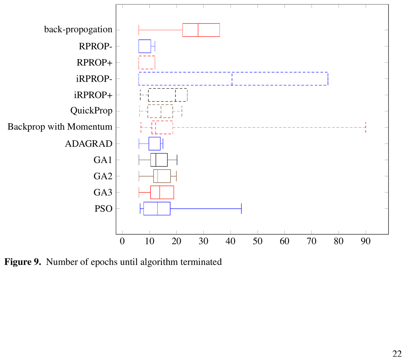
Report Figure 9, PDF p. 24 (printed p. 22): epochs until termination, cancer, 9×4×2×2, all twelve algorithms, 30 trials each.
This is the plot that step 9 of the protocol is defending against. Backpropagation’s box sits comfortably between 22 and 37 epochs with no long tail; most of the RPROP family and ADAGRAD are tighter still, under 20. Then there’s iRPROP−, whose box looks just as tight as its siblings but has a whisker stretching to 76, and Backprop with Momentum, whose box is barely visible near 15 but which has one trial that ran to 90. Average those in with the other 29 and you’d never notice the outlier existed; plot them as a box-and-whisker and it’s the first thing you see. That’s the entire argument for step 9’s “clip to the upper quartile” rule on the line plots: without it, the one 90-epoch Momentum trial would have stretched every other algorithm’s convergence curve out along the x-axis until they all looked flat.
And this is what 288 of these look like, one per dataset/algorithm/architecture combination, PDF pp. 62–349:
Every appendix page from the report, shrunk to a thumbnail and tiled. None of it is meant to be read at this size, it’s meant to be looked at as a wall. The whole point of the summary figures above is that nobody, including me in 2018, was reading all 288 of these page by page.
What it found
That last sentence is the actual sanity check underneath every post in this series: Prechelt published reference numbers for these exact datasets and architectures, and the report’s own runs land near them. Everything after that (iRPROP+‘s speed, QuickProp’s instability on gene, GA/PSO trailing the gradient methods) is consistent with a harness that’s actually measuring what it claims to.
I’d get to the discipline that made 3,960 training runs finish in reasonable time in
its own post: SpeedTests/SpeedTest1.py through SpeedTest16.py are sixteen
self-contained timeit scripts that never made it into the report at all, each
isolating one NumPy idiom (bias-as-row versus bias-as-vector, np.dot versus
np.einsum, method-call overhead) against an alternative. That post is
here, re-run on current NumPy with none of the original
numbers, since, as with everything else on this page, they were never written down.
Try the rule yourself
The 30-trial box plots above are the report’s, not something I can hand you a slider for. What I can hand you a slider for is the rule that decided when every one of those 3,960 runs stopped, which is arguably the more useful thing to actually understand: it needs no dataset, and it’s the part of this study most likely to show up again in your own training runs.
Pick a curve shape, or paste your own two columns of numbers, and drag α. The top panel is training and validation error against epoch; the bottom panel is and against the same epoch axis, plotted so the criterion firing is the point where the two lines cross. Watch the crossing point slide from stopping in the first few epochs, taking training error that’s still visibly falling with it, to never firing at all across a curve that overfit for a hundred epochs unchallenged.
With JavaScript on, this becomes an interactive simulator: pick a curve shape (clean convergence, a noisy validation split, a late overfit, or a plateau that resumes falling) or paste your own training and validation error, then drag α and the strip length k and watch where PQα would have stopped that run, with GL(t) and α·Pk(t) traced underneath and a readout of epochs wasted and how much validation error the stop cost you.
Two things worth doing in it. Switch to “plateau, then a second descent” and leave
α at 0.5: the criterion fires during the flat stretch, before the curve resumes
falling, because has nothing left to protect a run that has genuinely stopped
improving yet, even though it hasn’t stopped improving overall. There is no value of
α that fixes this without also making the criterion tolerate a real late overfit for
much longer, which is the actual, structural trade-off PQα is making, not a bug in it.
Then switch to “late overfit” and push k up past about 15: a strip that long starts
including training-error history from before the overfitting began, so stays
inflated and the criterion waits far longer than it should, training well past the true
best validation error. RPROPMnist.py’s bug, covered
here, was k fifty times too short; this is what
k too long costs instead, and both directions are one arithmetic slip away in a real
implementation.
What I take from it now
The methodology in this post is more careful than I expected to find when I went back and actually read §11 rather than skimming to the results, and PQα is the part of it I’ve kept using since. It’s a genuinely good answer to a question that’s easy to dodge: “training error keeps going down, so when do I stop?” isn’t answered by “when validation goes up,” because validation always goes up a little, constantly, from noise alone. It’s answered by weighing that uptick against how much the model is still learning, which is exactly the comparison makes.
It’s also a criterion with exactly one knob that matters (; mostly wants to be “long enough that noise averages out, short enough that it doesn’t smear over a real plateau”, and 5 epochs is a reasonable default rather than a carefully tuned one) and that knob has an honest, visible cost in both directions, which the widget above makes considerably harder to miss than a page of numbers ever did. Post 15 found what happens when the arithmetic behind that one knob is wrong by a factor of fifty. This post is what it looks like when the arithmetic is right, and eleven algorithms get to be compared on genuinely equal footing because of it.
Next in this series: I go back to that MNIST run, where the same criterion, computed one file differently, stopped training after a single epoch, and a naive Bayes classifier from the previous assignment won by nineteen points.