Blog · Neural networks from scratch ·
QuickProp, ADAGRAD and Momentum: three ways to guess a learning rate
Three different bets about the error surface: fit a parabola and jump to its vertex, shrink each step by how far it has already moved, or just keep going. Two of them work. Then QuickProp blows up, because it does.
- Interactive
- neural-networks
- optimisation
- quickprop
- adagrad
- momentum
- numpy
Last time, RPROP threw away the magnitude of the gradient entirely and kept only its sign. The next three algorithms in the report go the other way: each one is a different bet about what the gradient’s size is telling you. QuickProp bets that the error curve is a parabola and jumps straight to its vertex. ADAGRAD bets that a weight which has already moved a long way should take smaller steps from now on. Momentum bets nothing in particular: it just keeps some of whatever it was doing last time.
Two of the three are solid, boring, and outperform plain backprop with fewer knobs to tune. The third is the most interesting failure in the whole assignment.
QuickProp: fit a parabola, jump to the bottom
Quickprop’s assumption (report §6, PDF pp. 13–14, printed pp. 11–12) is that the error with respect to a single weight looks like a parabola, and that moving one weight barely disturbs the error contributed by any other weight, so each weight can be optimised as if it lived alone on its own one-dimensional curve:
Differentiate, and set the derivative to zero at three points in time: the vertex condition applied at , and the not-yet-known :
Two consecutive gradients are enough to solve for the parabola’s curvature, , since cancels between Eqns 6.2 and 6.3:
and falls out of Eqn 6.2 once is known:
Substituting both into Eqn 6.4 and solving for gives the whole algorithm in one line: jump directly to the vertex of the fitted parabola:
No learning rate anywhere in that formula. If the error really is a parabola in this weight, one step lands exactly on the minimum. That is the appeal, and it is also exactly where it breaks: the moment stops being smaller than , the denominator shrinks towards zero and the proposed step towards infinity. The report’s fix is a clamp, , on how much bigger this step is allowed to be than the last one, plus a fallback to plain backprop whenever the two-point fit can’t be trusted yet:
procedure QuickPropagation(input Matrix, Target Matrix, η, µ)
  for each w in the neural network's weights do:
    E'(t) ← the gradient associated with the current weight.
    Scale ← E'(t) / (E'(t − 1) − E'(t))
    Scale ← clip(Scale, −µ, µ)
    Δw(t − 1) ← Scale · Δw(t − 1)
    if sign(E'(t − 1)) == sign(E'(t)) or E'(t − 1) < 1e−15 then
      Δw(t − 1) ← Δw(t − 1) − η E'(t)
    end if
    w(t) ← w(t − 1) · Δw(t − 1)
  end for
end procedure
(That last line is printed with a ”·” in the report, PDF p. 14, printed p. 12: it should be ”+”, matching Eqn 6.7 and the actual code below. A transcription slip, not an algorithmic one.)
The supplementary backprop step fires whenever the two most recent gradients agree in
sign, meaning the curve hasn’t turned over between them, so there’s no vertex to jump
to yet, or whenever the previous gradient is too small to trust. The real code,
Classes/QuickProp.py:QuickPropLayer.backwardPropagate, lines 42–64:
dEdW = np.dot(deltaM.T, self.prevX).flatten()
dEdBias = np.sum(deltaM, axis=0).flatten()

scale = np.nan_to_num(dEdW/(self.pdEdW-dEdW))
np.clip(scale, -self.mu, self.mu, scale)
self.pDw = scale*self.pDw
inds = np.where(np.logical_or(np.sign(dEdW)==np.sign(self.pdEdW), self.pdEdW<1e-15))
self.pDw[inds] -= learningRate*dEdW[inds]

self.pdEdW=dEdW.copy()
self.pdEdBias=dEdBias.copy()
self.WeightMatrixT.flat += self.pDw
self.BiasVector += self.pDbias
self.pDw and self.pdEdW are both zero-initialised, which is what makes the very first
update reduce cleanly to plain gradient descent: self.pdEdW < 1e-15 is true when
pdEdW is still zero, the supplementary branch fires for every weight, and the
quadratic-fit term is scale * self.pDw = scale * 0 = 0 anyway.
ADAGRAD: shrink the step by how far you’ve already moved
ADAGRAD (report §7.1, PDF p. 14, printed p. 12, Algorithm 8) keeps a running sum of squared gradients per weight and divides the learning rate by its square root, so a weight that has already accumulated a lot of gradient takes smaller steps from then on:
procedure ADAGRAD(input Matrix, Target Matrix, η)
  Forward propagate each input and store Z^(m-1) and Z^(m) for each layer m, m ← 1 to M
  errorContrib ← Σ_{inputs,targets} (Z^(M) − t)
  gτ ← 0
  for m from M down to 1 do
    Calculate δ^(m) using Eqn. 4.14.
    ∂E/∂W^(m) ← gradient associated with each weight.
    gτ ← gτ + (∂E/∂W^(m))²
    W^(m)(t+1) ← W^(m)(t) − (η / √gτ) · δ^(m) · (Z^(m−1))ᵀ
    errorContrib ← W^(m) · δ^(m)
  end for
end procedure
The actual layer, Classes/MomentumLayer.py:NetworkLayerWithAdaptiveWeights.backwardPropagate,
lines 94–103:
deltaBiasM = -learningRate*deltaM

holdOut = np.dot(deltaM, self.WeightMatrixT)
holdDw = np.dot(deltaBiasM.T, self.prevX)

self.HdEdW += holdDw**2
self.HdEdBias +=np.sum(deltaBiasM, axis=0)**2

self.WeightMatrixT += (holdDw / (1e-10 + np.sqrt(self.HdEdW)))
self.BiasVector += (np.sum(deltaBiasM, axis=0) / (1e-10 + np.sqrt(self.HdEdBias)))
Reading that carefully turned up something I hadn’t noticed before: it isn’t quite
Algorithm 8. holdDw is already -η·∂E/∂W, the learning rate is baked in before it’s
squared and accumulated into self.HdEdW. So the accumulator holds
, not
as Algorithm 8’s line 8 says. Carry that
through the update:
for any not absurdly close to zero: the in the numerator and the inside the square root in the denominator cancel. That was a fun one to catch, so I checked it wasn’t just algebra that looks right: I ran the update in Python for five made-up gradients with (a 600× range), and the resulting weight after five steps agreed to nine significant figures every time.
The report’s own read on ADAGRAD (§13) is that it “had a similar performance to the backward propagation algorithm but had less parameters to tune”, which, given the finding above, is generous to backprop and exactly right about the tuning: there’s effectively nothing to tune.
Momentum: keep doing what you were doing
The plainest of the three (report §7.2, PDF p. 15, printed p. 13, Algorithm 9). Keep a fraction of the previous step and add it to the current one:
procedure Backward-Propagation-With-Momentum(input Matrix, Target Matrix, η, α)
  Forward propagate each input and store Z^(m-1) and Z^(m) for each layer m, m ← 1 to M
  errorContrib ← Σ_{inputs,targets} (Z^(M) − t)
  ΔW^(n) ← 0
  for m from M down to 1 do
    Calculate δ^(m) using Eqn. 4.14.
    ∂E/∂W^(m) ← gradient associated with each weight.
    ΔW^(n) ← −η δ^(m) · (Z^(m−1))ᵀ + α ΔW^(n)
    W^(m)(t+1) ← W^(m)(t) + ΔW^(n)
    errorContrib ← W^(m) · δ^(m)
  end for
end procedureClasses/MomentumLayer.py:NetworkLayerWithMomentum.backwardPropagate, lines 25–31, is a
faithful line-for-line match: no discrepancy to report here, a pleasant change:
deltaBias = -learningRate*deltaM

self.prevDW = np.dot(deltaBias.T, self.prevX) + self.Momentum*self.prevDW
self.prevDbias = np.sum(deltaBias, axis=0) + self.Momentum*self.prevDbias

self.WeightMatrixT += self.prevDW
self.BiasVector += self.prevDbias
Table 2’s matches MomentumTestProben1.py:95 exactly. Its learning-rate
row (“exponentially decays from 0.8 at epoch 1 to 0.005 at epoch 25”) is only true for
four of the six datasets. MomentumTestProben1.py:27–32 sets the decay’s starting value
per dataset: flare, gene, horse and heartc do start at 0.8, but cancer and card start at 2,
ten times higher than QuickProp’s own supposedly-2 learning rate turned out to actually be.
What the benchmark said
Each algorithm ran 30 times per dataset per architecture with PQ early stopping. Below is the gene dataset (120 inputs, 3 outputs, a 120×4×2×3 network), the case the report itself points to for QuickProp’s failure mode (§13, referencing §12.1.4).
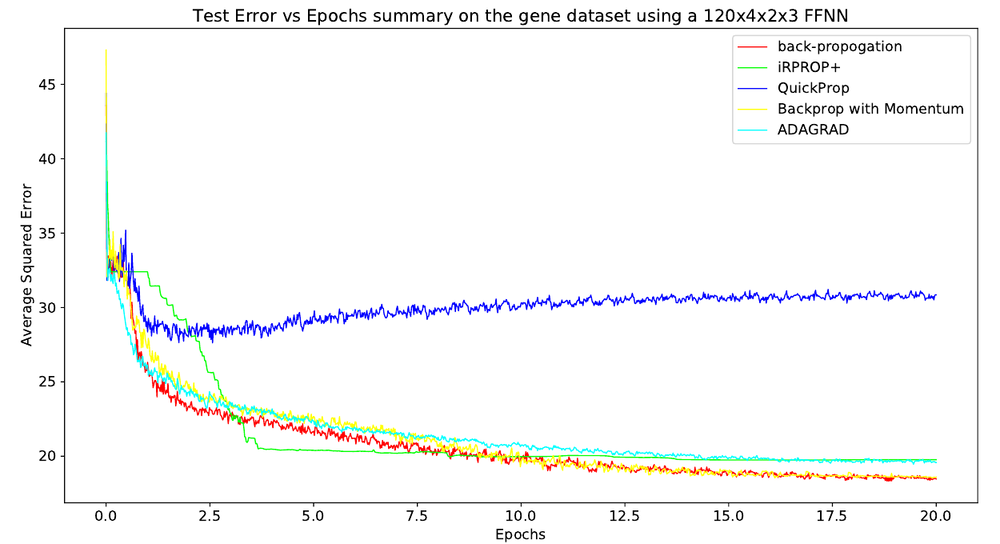
Report Figure 34, PDF p. 37 (printed p. 35). Average squared error percentage on the test set, gene dataset, 120×4×2×3, averaged over 30 trials. QuickProp (blue) is the only curve that goes back up.
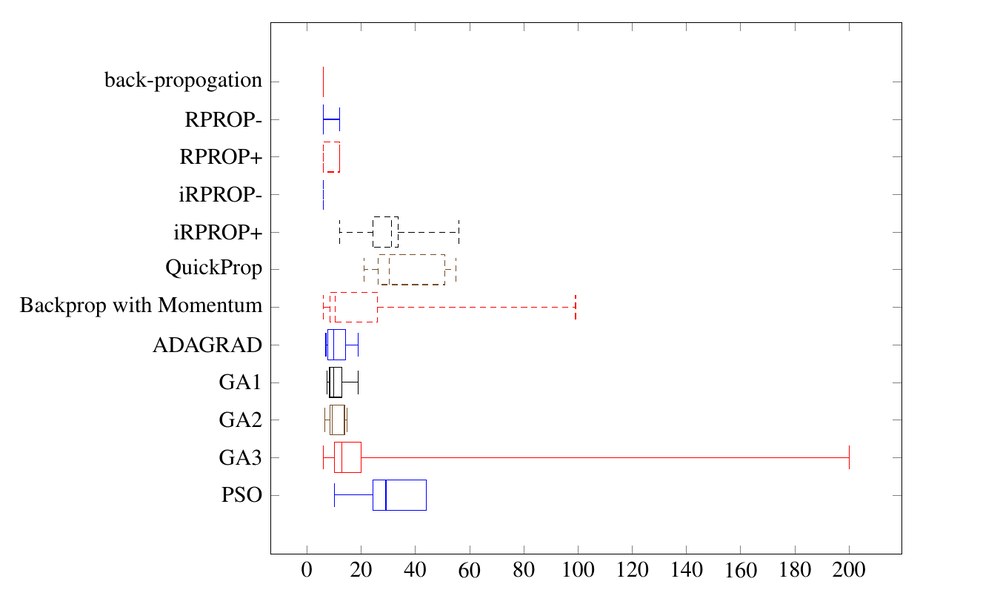
Report Figure 39, PDF p. 39 (printed p. 37). Epochs until PQ stopped training, same dataset and architecture, all eleven algorithms, 30 trials each.
On ADAGRAD and momentum, the same section: “The ADAGRAD algorithm had a similar performance to the backward propagation algorithm but had less parameters to tune… Adding momentum to the backward propagation does not affect performance much for small datasets like proben1. It does however make it more likely to reach a global minimum… Especially when there is less redundancy in the parameter space, such as in Sec. 12.1.2, one can see that backward propagation with momentum tends to achieve a lower error and a smaller test error range.”
Watch QuickProp fit its parabola
This is the picture that makes Eqns 6.5–6.7 click. Pick a surface, press Step. Each press samples the gradient at the current weight, draws it and the previous sample as two tangent lines, solves the one parabola through both (the dashed curve), and proposes a jump to its vertex. The faint arrow is that raw, unclamped jump; the solid one is what actually happens once truncates it and, often, a plain backprop nudge is added on top.
With JavaScript on, this becomes a step-by-step panel: pick a clean quadratic, a quartic with two minima, or a noisy surface, and step through QuickProp fitting a parabola to two sampled gradients and jumping toward its vertex, with a µ slider that physically shortens the jump.
On the clean quadratic, QuickProp’s assumption is exactly true: after the first (plain-backprop) step, the second step’s fitted parabola is the real curve, and it lands on the minimum in one move regardless of . On the quartic, watch what happens when the two sampled gradients straddle the local maximum between the two minima: the fitted parabola opens the wrong way (negative curvature), its “vertex” is a maximum, and the proposed jump can point away from both minima entirely. On the noisy surface, two nearby points can produce a wildly different curvature estimate from one step to the next, which is the mechanism behind the gene-dataset plot above: not one bad step, but the estimate itself being unreliable on anything that isn’t a clean bowl.
The same race, four algorithms
Post 7’s contour racer, unchanged, with the four RPROP variants swapped for plain gradient descent, momentum, ADAGRAD and QuickProp. Drag the start point, tick the algorithms you want, and watch what each one’s bet about the surface actually buys it, including QuickProp leaving the plot.
With JavaScript on, this becomes an interactive race: gradient descent, momentum, ADAGRAD and QuickProp on a contour plot you can drag the start point around, with per-algorithm learning-rate sliders and a “learning-rate roulette” game underneath.
Set above about 1.5 on Beale or the double well and QuickProp reliably shoots off the edge within a handful of steps: the corner gradients there are enormous, two consecutive samples rarely have similar magnitude, and the scale ratio keeps slamming into the clamp in the same direction. Turn down toward 0.1 and QuickProp behaves like a nervous, slow gradient descent that never trusts its own curvature estimate enough to speed up.
The “learning-rate roulette” button drops the shared start point somewhere random on the surface and asks you to guess which algorithm gets to the minimum first, before it plays out automatically; the little table underneath keeps score across rounds. On Beale, gradient descent and ADAGRAD win the most rounds in my own testing; QuickProp either wins spectacularly fast, when the corner gradients happen to hand it a good curvature estimate, or diverges and is disqualified. That is the whole algorithm in miniature.
Table 2, transcribed
The report’s summary of every hyperparameter actually used (PDF p. 19, printed p. 17): the three rows this post concerns, exactly as printed:
| Algorithm | Parameters |
|---|---|
| QuickProp | , |
| ADAGRAD | |
| Backward propagation with momentum | exponentially decays from 0.8 at epoch 1 to 0.005 at epoch 25 and higher; |
Two of those three rows, as the callouts above show, are not what the code actually ran.
What I take from it now
QuickProp’s failure is a clean illustration of what happens when an algorithm’s whole
identity rests on one assumption that isn’t checked at runtime: nothing in
QuickPropLayer.backwardPropagate ever asks whether the last two gradients actually came
from something parabola-shaped. It just fits the parabola through whatever two points it
has and jumps, every time, and trusts to catch the worst of it. On the gene dataset
that produces exactly the shape in Figure 34: a fast initial drop, because the first few
steps genuinely are close to quadratic near a cold start, followed by a slow climb once the
curvature estimate stops being trustworthy and the clamp is doing all the work.
ADAGRAD and momentum earn their reputations honestly here, and ADAGRAD earns it almost by accident. The report frames it as “a similar performance to backprop with less parameters to tune,” and the code makes that truer than intended, since one of its two parameters barely does anything. Two decades on, Adagrad’s per-parameter accumulator and the running average that Adam builds on top of it are still the dominant idea in how optimisers are built; QuickProp’s second-order bet mostly wasn’t, outside of a few specialised uses. Fast when its assumption holds, and this post’s whole point, unstable when it doesn’t, was apparently not a trade the field wanted to make twice.
Next in this series: the same contour, but with a population of 64 creatures on it instead of a single point, for the genetic algorithms and particle swarm optimisation.