Blog · Neural networks from scratch ·
Training a neural network without gradients: genetic algorithms and PSO
Flatten every weight into one vector, evaluate sixty-four candidate networks in a single tensor contraction, and breed them. It loses badly to backprop, and why it loses is the whole lesson.
- Interactive
- neural-networks
- optimisation
- genetic-algorithms
- particle-swarm
- numpy
The last three posts were all arguments about the gradient. Backprop computes it, RPROP throws away everything but its sign, and QuickProp, ADAGRAD and momentum each make a different bet about what its magnitude means. Every one of them needs the derivative to exist and needs you to be able to write it down.
The last two algorithms in the assignment need neither. Take every weight and bias in the network, flatten them into one long vector, and call that vector a creature. Make sixty-four of them at random. Score each one by running the training set through it. Then either breed the good ones and mutate the children (a genetic algorithm), or give each one a velocity and let them chase each other toward the best position anyone has found (particle swarm optimisation). Neither ever differentiates anything.
They lose. Badly. The report’s own conclusion (§13, PDF p. 59, printed p. 57) is blunt about it: “GA and PSO perform significantly worse than the gradient based algorithms. This is expected as the gradient based algorithms are able to exploit the geometry of the search space.” That sentence is the whole post. A gradient tells you which way is downhill from where you are standing, for free, in one backward pass. A population has to discover that by sampling, and sampling in a few hundred dimensions is a hopeless way to learn a direction.
But watching them fail is unusually instructive, because every design decision in a genetic algorithm is visible on a two-dimensional plot in a way that a gradient step never is.
Weights as a genome
The network doesn’t change at all. NeuralNetwork.getSizeOfWeightVector
(Classes/NeuralNetworkClass.py:278) already knows how many numbers a given topology needs:
return np.sum((np.array(layerNeurons[:-1])+1)*layerNeurons[1:])the being each layer’s bias. For the 9×4×2×2 network the report uses on the cancer dataset that is 56 numbers; for the 3×40×3 counter in the unit tests it is 283. Whatever it is, it is a point in , and any search method that can optimise a function of real numbers can train the network.
The interesting engineering is one line. Evaluating a population means forward-propagating
64 different networks over the same batch of training rows, and in NumPy a Python loop over
64 creatures would dominate everything. batchNetworkLayer.forwardPropagate
(Classes/NeuralNetworkClass.py:399) doesn’t have one:
return 1.0/(1.0+np.exp(-np.einsum('kji, kli->klj', self.WeightMatrixT, inputMatrix)-self.BiasVector))k indexes the 64 candidate networks, l the rows of the training batch, and i/j the
layer’s fan-in and fan-out. One contraction propagates every creature over every row
simultaneously. The whole population lives in one contiguous buffer: BNN.weights.view() in
each runner is a (64, D) view onto it, so the genetic algorithm mutates weights by
indexing straight through with WeightMatrix.flat[...] and the network sees the change
without anything being copied. That is what makes 11 algorithms × 6 datasets × 2
architectures × 30 trials finish on a laptop.
The error per creature is the other half (getBatchError, L520–535):
outputmatrix = self.forwardPropagate(inputMatrix)
return np.sum((outputmatrix-targetMatrix)**2, axis=(1, 2))
Sum of squares over rows and outputs, collapsed to one number per creature. That vector of 64 errors is the only thing the GA and the swarm ever see about the network.
Selection: take the best, or roll a weighted die
Report §8.1 (PDF p. 16, printed p. 14) sets up the choice. The simple method takes the top by error, and is cheap precisely because the don’t have to be ordered. The alternative samples creatures without replacement with probability proportional to inverse error, which “allows for slightly worse creatures to be selected” and is therefore “less likely to get stuck on local minima”.
Both are four lines. Classes/GeneticAlgorithmMatrix.py:30–39:
def SelectionProbabilityWeights(seeds, error, selectionSize):
    inverseError=1.0/(error+0.000001)
    return seeds[np.random.choice(np.arange(len(seeds)),
                                  size=selectionSize,
                                  replace=False,
                                  p=inverseError/np.sum(inverseError))]

def TopN(seeds, error, selectionSize):
    indicies=np.argpartition(error, selectionSize)[:selectionSize]
    return seeds[indicies]
np.argpartition is the “don’t have to be ordered” observation cashed in: it’s where
a sort is , and it hands back the smallest in arbitrary order. The
in the other function is the “small twiddle factor… to allow numeric stability” the report
mentions; without it a creature that fits the training set exactly divides by zero and takes
the entire probability mass.
There is a third function, TopNSorted (L41–43), which argsorts the errors of the
partitioned subset and then uses those ranks as indices into seeds, so it returns the
first creatures in the population regardless of their error. It is broken, and it is also
dead: nothing in the repo calls it.
Crossover: the decision that shows up on the plot
This is the one worth drawing. Both crossovers split a genome in half at
weightMidway = int((chromesoneLength+1)/2.0) and glue one parent’s head to another parent’s
tail. They differ in which pairs get made.
allCombos (L53–63) makes every pair. To keep the population at you therefore need
exactly parents (the assert on L56 says so out loud), which for means
eight parents produce all sixty-four children:
self.selectionCount=np.sqrt(numberOfSeed)
assert float(self.selectionCount).is_integer(), "The population size must be a squared number"
...
def Crossover(self, WeightMatrix, SelectedSeeds):
    holdStart=np.repeat(SelectedSeeds[:,:self.weightMidway],self.selectionCount,axis=0)
    holdEnd=np.tile(SelectedSeeds.T[self.weightMidway:],self.selectionCount).T
    WeightMatrix[:]=np.append(holdStart,holdEnd,axis=1)
The repeat/tile pair is the outer product written in index gymnastics: child gets
parent ‘s head and parent ‘s tail. The report’s objection (§8.2) is that this “lessens
the diversity of the population as a small set of the overall population must be selected”
and that “a single gene in the parent has influence over a large population of the child
genes”, one parent’s head appears in eight of the sixty-four children.
_2NearestNeighborsCrossover (L65–77) pairs consecutive parents in a circular array instead,
giving two children per parent, so : thirty-two of the sixty-four survive to
breed:
def Crossover(self, WeightMatrix, SelectedSeeds):
    WeightMatrix[:,:self.weightMidway]=SelectedSeeds[:,:self.weightMidway].repeat(2,axis=0)
    aend=SelectedSeeds[:,self.weightMidway:]
    WeightMatrix[::2,self.weightMidway:]=np.roll(aend, 1, axis=0)
    WeightMatrix[1::2,self.weightMidway:]=np.roll(aend, -1, axis=0)
Child takes parent ‘s head with parent ‘s tail; child takes the same head with parent ‘s tail, wrapping at the ends.
Now the part that makes this drawable. On a two-dimensional landscape a genome is
, weightMidway is 1, and “head” and “tail” mean literally “the x coordinate” and
“the y coordinate”. So allCombos on a 2-D problem produces every combination of eight
selected s with eight selected s, the entire population snaps onto an 8×8 lattice you
can see. nearest2 produces 64 scattered pairs from 32 parents. The abstract argument about
diversity turns into a picture of a grid collapsing.
Mutation, and the annealing that never happens
Report §8.3: select chromosomes from the whole population, add ,
and shrink by a factor each generation down to a floor
, so the search is “more random at the start and more selective when closer
to an optimal solution”. SimpleMutation and DampedMutation, L80–98:
class SimpleMutation:
    def __init__(self, numberOfSeeds, chromesoneLength, numberToMutate, mutationValueStd):
        self.numberToMutate=numberToMutate
        self.mutationValueStd=mutationValueStd
        self.GeneCount=numberOfSeeds*chromesoneLength

    def Mutation(self, WeightMatrix):
        MutationIndicies=np.random.randint(0,self.GeneCount,self.numberToMutate)
        WeightMatrix.flat[MutationIndicies]+=np.random.normal(0,self.mutationValueStd,self.numberToMutate)

class DampedMutation(SimpleMutation):
    ...
    def Mutation(self, WeightMatrix):
        super().Mutation(WeightMatrix);
self.mutationValueMean=max(self.mutationValueStd*self.dampingConst,self.minStd)Two smaller things in the same neighbourhood. np.random.randint draws with replacement,
so “mutate 5% of the genes” actually mutates slightly fewer than 5% distinct genes, some of
them twice. And Table 2 writes the mutation parameters as variances, ,
, while the code passes them to np.random.normal(0, ...), whose
second argument is the standard deviation. For the initial value it makes no difference,
since ; for the floor it is the difference between and , and since the
floor is never reached anyway, it doesn’t matter either.
The four variants
Two binary decisions, four cells. GA2TestProben1.py and GA3TestProben1.py are byte-for-byte
copies of GA1TestProben1.py apart from the algName string on line 10 and exactly one of
lines 99–101: GA2 swaps GA.TopN for GA.SelectionProbabilityWeights, GA3 swaps
GA.allCombos for GA._2NearestNeighborsCrossover. That is the whole experiment.
| All combinations (8 parents) | Nearest 2 (32 parents) | |
|---|---|---|
| Simplistic (top M) | GA1 | GA3 |
| Probabilistic (1/error) | GA2 | GA4, not in the report |
There is one more quirk shared by all four runners, worth knowing before you read the plots:
after the first trial, the generation budget for the remaining 29 is set from how long trial
zero took (GA1TestProben1.py:151–152):
if (Trial==0):
    generationCount=max(ceil(epoch*2),generationMinCount)
generationCount starts at 2,000, and the assignment happens inside the running loop, so
the moment PQ fires at generation in the very first trial, that trial and all 29
after it are capped at . That is why the GA curves below stop after thirteen generations
on cancer and after five on gene, rather than the two thousand the script nominally allows.
Watch a population breed
Sixty-four creatures on the same contour surfaces the last two posts raced single optimisers across. Press Play. Each generation, the previous population is drawn in place (a ring around anyone selected as a parent, a faint × over everyone culled) and the children land on top, with the ones that caught a mutation drawn larger and in the accent colour. The star is the best creature seen so far.
The one thing that changes from the previous two posts is the marker. A genetic algorithm has
no starting point: the runners seed every weight from np.random.uniform(-2, 2) and that is
the entirety of its initial state. So the population here is seeded uniformly across the whole
plotted surface and ignores the marker completely, which only matters in the third mode,
where gradient descent needs somewhere to stand.
With JavaScript on, this becomes a population of 64 creatures on a contour plot: pick the selection and crossover rules to build GA1, GA2, GA3 or the unpublished GA4, watch who breeds and who is culled each generation, and read the diversity collapse off a fitness histogram.
Switch crossover to All combinations and step a few generations on any surface. Eight parents, every combination of their heads and tails, and the population visibly lands on an 8×8 grid: every creature shares its with seven others and its with seven others.
Then drag the mutation p slider to 0% and press Reset. With nothing putting variation back, §8.2’s argument becomes a measurement. I ran all four variants 40 times each on the double well, 64 creatures, and recorded the mean pairwise distance across the population:
| Median population spread, no mutation | gen 1 | gen 3 | gen 10 | gen 30 |
|---|---|---|---|---|
| GA1: top M + all combinations | 0.70 | 0.00 | 0.00 | 0.00 |
| GA2: roulette + all combinations | 1.97 | 1.20 | 0.08 | 0.00 |
| GA3: top M + nearest 2 | 1.51 | 0.53 | 0.00 | 0.00 |
| GA4: roulette + nearest 2 | 2.02 | 1.79 | 0.52 | 0.14 |
GA1 is down to a single point by generation three. Eight parents chosen by truncation, crossed with each other in every combination, and after two rounds all eight are the same creature: the 8×8 lattice degenerates to one cell and the algorithm is finished. GA3 buys seven more generations by breeding 32 parents instead of 8; GA2 buys about thirty by letting worse creatures into the parent pool; only GA4, which does both, still has any spread left at generation 30. That is exactly the ordering §8.2 predicts, and it is invisible in the report’s plots because mutation is never switched off in them.
Turn mutation back on and the picture changes character completely. At each variant’s own rate the spread stops falling and settles on a floor (0.16 for GA1 and GA3, 0.31 for GA2, 1.10 for GA4), and that floor is set almost entirely by the mutation rate and , not by the crossover. Mutation isn’t adding diversity at the margin here; it is the only thing holding the population apart at all. Which puts a different weight on the annealing bug above: with pinned at 1 forever, the GA can never stop jittering and settle, and with the annealing working it would have collapsed to whatever crossover left it.
So which variant is best? On the evidence in the report, not the one §8.2 argues for.
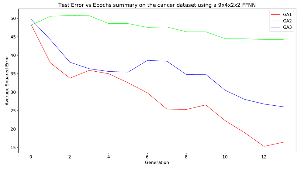
Report Figure 6, PDF p. 23 (printed p. 21). Test error against generation, cancer dataset, 9×4×2×2 network, averaged over 30 trials. Note the axis: the plot title says “vs Epochs” and the x-axis says “Generation”, for a GA those are not the same thing, and one generation costs 64 forward passes where one epoch costs one.
GA1 (eight parents, a lattice that has collapsed to a point by generation three if mutation doesn’t refill it) is comfortably the best of the three, and GA2 barely learns at all. Thirteen generations is not much of a test, and cancer is the easiest of the six Proben1 datasets, but it is what the report has, and my own re-runs on the binary counter further down agree with it: GA1 first, GA3 close behind, GA2 a long way back.
My reading now is that over thirteen generations there is simply no time for diversity to pay off. Truncation selection’s much faster early progress is all that gets measured, and the argument in §8.2 is about a regime the experiment never reaches. It is the sort of thing 200 trials of GA4 might have settled.
Particle swarm: everybody chases the leader
Report §9 (PDF p. 17, printed p. 15). Each particle keeps a velocity, remembers the best position it has personally visited, and is pulled toward both that and the best position anyone has visited. Algorithm 10, transcribed:
procedure PSO(Φg, Φp, ω, Initial particle positions, Position Range)
  particlePositions ← Initial particle positions
  bestPositions     ← Initial particle positions
  bestValues        ← Error score for each particle at current position.
  globalBestIndex   ← index of the lowest value in bestValues.
  V ← U(−Position Range, Position Range)
  while not converged do
    for each particle p do
      r_p ← U(0, 1)
      r_g ← U(0, 1)
      V ← ωV + Φp·r_p·(bestPositions[index_p] − particlePositions[index_p])
             + Φg·r_g·(bestPositions[globalBestIndex] − particlePositions[index_p])
      particlePositions[index_p] ← particlePositions[index_p] + V
      error ← error of particle at current position.
      if error < bestValues[index_p] then
        bestValues[index_p]  ← error
        bestPositions[index_p] ← particlePositions[index_p]
        if error < bestValues[globalBestIndex] then
          globalBestIndex ← index_p
        end if
      end if
    end for
  end while
end procedure
Or, for particle with position , personal best and global best :
with drawn fresh every step. Table 2 takes and from reference [17], Poli, Kennedy and Blackwell’s 2007 survey: the standard constriction-derived pair, and the numbers everybody uses.
(Two liberties in that transcription. The printed line 17 reads
if error < bestValues[globalBestIndex with the bracket unclosed, which I have closed. And
V is written as a single variable for the whole swarm, where it plainly has to be one
velocity per particle, the code gets that right, so I have not carried the slip through. The
algorithm is also written asynchronously: each particle moves and is re-scored inside the
per-particle loop, so a particle late in the loop already sees the global best updated by one
earlier in it. The code is synchronous: it scores the whole population, then moves the whole
population. Both are standard variants of PSO; they are not the same algorithm.)
The implementation is thirty-seven lines. Classes/PSO2.py:15–29:
def iterate(self, inputData, targetData, weights):
    currentError=self.getError(inputData, targetData)
    minInds=np.where(currentError<self.bestVals)[0]
    self.bestVals[minInds]=currentError[minInds]
    self.bestPos[minInds,:]=weights[minInds,:]

    self.globalbestIndex=np.argmin(self.bestVals)

    r_p=np.random.uniform(0,self.Phi_p,weights.shape)
    self.r_g=np.random.uniform(0,self.Phi_g,weights.shape)

    self.particalVelocity=self.omega*self.particalVelocity+r_p*(self.bestPos-weights)+r_p*(self.bestPos[self.globalbestIndex]-weights)
    weights+=self.particalVelocity
Drawing from rather than multiplying by is the same thing, and the whole update is one vectorised expression over all 64 particles at once, which is neat. Line 26 is not neat.
The widget below runs both. Because the buggy line still draws self.r_g before discarding
it, a faithful swarm and a buggy swarm started from the same seed consume exactly the same
random numbers in the same order, so “both, same seed, side by side” is a genuine controlled
experiment with one variable in it.
With JavaScript on, this becomes a 64-particle swarm on a contour plot with velocity arrows, personal-best ghosts and a starred global best, plus a switch between the repo’s velocity update, the one Algorithm 10 prints, and both at once from the same random seed.
Run both on the double well and press Play. For the first twenty or so steps they are hard to tell apart, the enormous starting velocity dominates and both swarms are flying. The difference is in the endgame, and it is not the one I expected when I first read line 26. The faithful swarm contracts: after 120 iterations its mean pairwise spread is about 0.003, i.e. all 64 particles are sitting on the answer. The buggy swarm never settles at all: same measurement, 32, particles still scattered across an area many times the size of the plot, orbiting a global best that stopped improving long ago. Both numbers are medians over 40 runs, and all four surfaces give the same story.
The reason is in the variance rather than the mean. Write the total acceleration coefficient as the thing multiplying the pull toward the attractor. Algorithm 10 has with independent; the repo has . Both have the same expectation, 1.49618, but where . The bug leaves the average pull alone and doubles its variance, and a swarm whose step size fluctuates twice as hard doesn’t damp out. So the shipped PSO explores more than it should and converges less than it should, which on a two-dimensional plot with 64 particles costs almost nothing (the best-so-far marker still lands on the minimum), and in 283 dimensions, as the next section shows, costs a great deal.
The third button on either widget puts all three methods on one surface with a finish line drawn at 1% of the plot diagonal from the nearest minimum. The swarm wins almost every surface, usually inside thirty generations, which is §13’s “PSO … is able to converge at a faster rate than the genetic algorithm” reproduced on a toy. GA1 only finishes on the double well; on Rosenbrock, Beale and the valley it is still refining when the 300-generation budget runs out, and you have to reach for GA4 or a bigger mutation to change that.
Gradient descent has a learning-rate slider in that mode, because it needs one. At it reaches the double well’s minimum in about 160 steps and diverges outright on Rosenbrock and Beale, where you have to drop it to 0.002 and then it is far too slow to finish inside the budget. Neither the genetic algorithm nor the swarm has a step size to tune at all. That is a real advantage, it is the one people usually mean when they reach for these methods, and the next section is about what it costs.
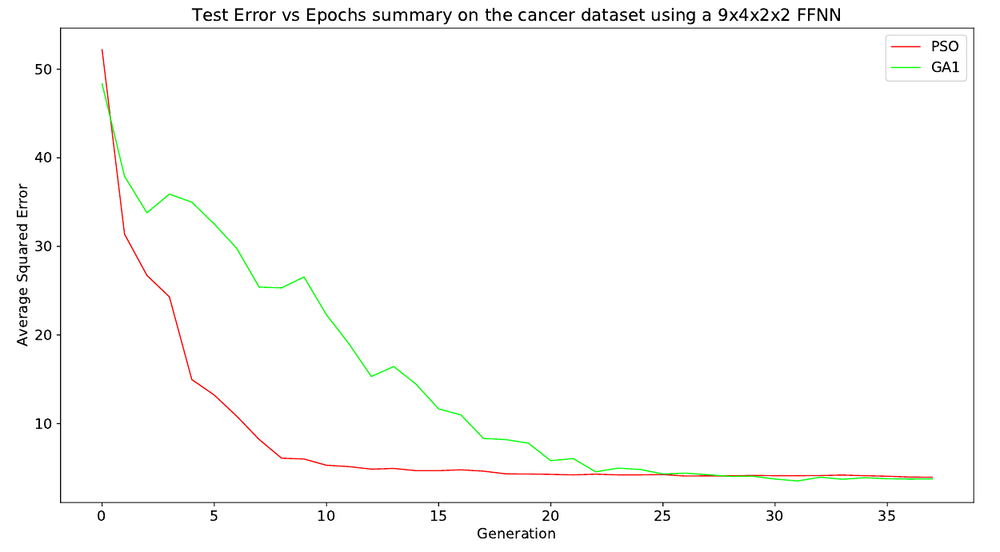
Report Figure 7, PDF p. 23 (printed p. 21). PSO against GA1, cancer dataset, 9×4×2×2, 30 trials. Same “vs Epochs” title over a “Generation” axis as Figure 6.
Figure 7 shows the first half of that claim clearly enough: PSO is at error 5 by generation 8 where GA1 needs 22. The second half, the plateau, doesn’t show on cancer, where both end up around 4. It shows on gene:
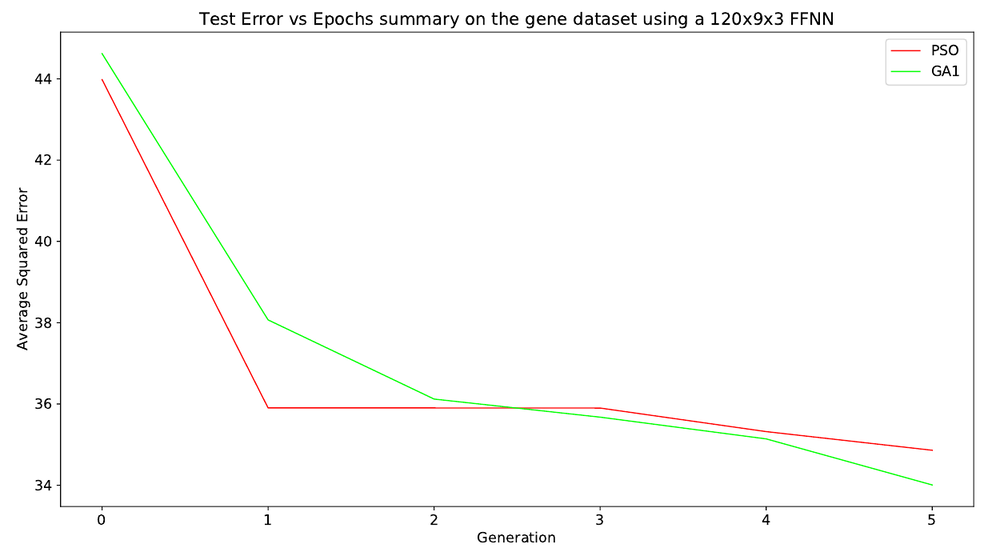
Report Figure 49, PDF p. 44 (printed p. 42). PSO against GA1, gene dataset, 120×9×3, 30 trials. PSO is flat at 35.9 from the first generation onward; GA1 keeps descending, crosses it between generations 2 and 3, and finishes lower.
That is §13’s sentence rendered as a picture: PSO gets there faster, stops, and is passed. Whether the stopping is PSO’s or line 26’s, the report has no way to know and neither do I, except that on the binary counter below, where I can run both, the faithful swarm solves the problem in a third of the generations and the shipped one fails outright in seven runs out of twenty.
The bit that actually settles it
Contour plots are a good way to see how these algorithms move and a bad way to see how badly they lose, because a two-dimensional problem is exactly the case where random search is fine. So here is the repo’s own toy network instead.
UnitTests/GA_BinCountTest.py and UnitTests/PSO_BinCountTest.py both train a 3×40×3
sigmoid network to map a three-bit number to its successor, wrapping 111 back to 000. Eight
training rows, 283 weights, no dataset to download. Below it runs in your browser, with the
population methods and full-batch backpropagation on the same architecture, the same eight
rows and the same error measure.
With JavaScript on, this trains the repository’s own 3×40×3 binary-counter network three ways at once (a genetic algorithm, a particle swarm and backpropagation), plots training error against generation on a log scale, and shows the eight-row truth table each method’s best network currently produces. There is no figure for it in the report: the binary counter appears only in the unit tests, whose output was never saved.
I also ran it offline, 20 seeds per method, stopping the moment the best network gets all eight rows right when thresholded at 0.5:
| Method | solved within 1,500 steps | median steps | median batch forward passes |
|---|---|---|---|
| GA1 | 20/20 | 56 | 3,584 |
| GA2 | 6/20 | 735 | 47,040 |
| GA3 | 19/20 | 129 | 8,256 |
| GA4 | 17/20 | 440 | 28,160 |
| PSO: the repo’s line 26 | 13/20 | 785 | 50,240 |
| PSO: Algorithm 10 | 20/20 | 248 | 15,872 |
| Backpropagation, | 20/20 | 197 | 197 |
(Medians are over the runs that got there; a step is one generation for the population methods and one full-batch epoch for backprop. These are my numbers from re-running the ported code, not the report’s, there are no published results for the binary counter.)
Three things fall out of that table. GA2 is the worst by a distance, failing 14 runs out of 20, which is an independent confirmation of Figure 6, where GA2 is the curve that barely moves. The PSO bug costs a factor of three in generations and seven failures out of twenty: the shipped swarm is meaningfully worse than the algorithm the report describes, and every PSO number in the 349 pages was produced by the shipped one. And counted in generations, the genetic algorithm looks competitive: GA1’s median 56 generations beats backprop’s 197 epochs outright.
Then tick “x-axis counts forward passes” and the whole thing inverts. One GA generation is 64
batch evaluations, because that is what evaluating 64 creatures costs, no matter how elegant
the einsum is. On equal compute GA1 needs 3,584 forward passes to backprop’s 197, an
18-fold gap on the easiest problem in the repository, against the best of the four GA
variants, on a network with 283 weights. There is no reason to expect that to shrink as the
network grows: whatever the dimension, a generation still buys the population exactly 64
numbers, while a backward pass buys backprop one partial derivative per weight.
That is the lesson stated as sharply as I can state it. The gradient is not a heuristic for finding downhill; it is downhill, delivered by a backward pass that costs about what the forward pass did. Sampling 64 points and keeping the good ones is a very expensive way to estimate the same information, and the estimate is bad: one scalar per creature, against a 283-component vector that says exactly which way each weight should move. Everything the population methods have going for them, and it is a real list (no derivative needed, no smoothness needed, no chain rule to get wrong, trivially parallel) is worth nothing on a problem where the derivative exists and is cheap.
Where they are not worth nothing is where the derivative doesn’t exist. That is the honest frame for this pair of algorithms, and it is not a frame that an optimiser benchmark on feed-forward networks can show you.
Table 2, transcribed
The GA and PSO rows of the report’s hyperparameter table (PDF p. 19, printed p. 17). The values are as printed; I have only folded each cell’s four lines onto one, and written “as GA1” for the mutation clause, which is character-for-character identical in all three GA rows:
| Algorithm | Parameters |
|---|---|
| GA1 | Number of creatures = 64; Selection: Simplistic; Crossover: All Combinations; Mutation: Select of chromosomes Gaussian with , and |
| GA2 | Number of creatures = 64; Selection: Probabilistic; Crossover: All Combinations; Mutation: as GA1 |
| GA3 | Number of creatures = 64; Selection: Simplistic; Crossover: Nearest 2; Mutation: as GA1 |
| PSO | Number of particles = 64; ; ; . “These parameters were chosen from [17]” |
What I take from it now
Two things, and neither is “genetic algorithms are bad”.
The first is that the design decisions in a population method are not tuning knobs; they are the algorithm. Selection and crossover between them decide how fast diversity drains out of the population, and that single quantity determines whether the run escapes a local minimum or dies in it. Eight parents versus thirty-two is not a small change: with mutation off it is the difference between a population that is a single point by generation three and one that is still spread out at generation thirty. And the report’s own results have the “wrong” one winning, because the runs were far too short for the difference to matter, which is its own lesson about benchmarks.
The second is about the bugs. Two of the three are one-token slips (mutationValueMean for
mutationValueStd, r_p for r_g), and both silently removed a mechanism the surrounding
prose spends a paragraph explaining; the third, iterateNextGeneration’s index into the wrong
generation, is four lines in the wrong order. None of them crashes. None produces a number
that looks wrong. The GA still converges, the swarm still swarms, the plots still look like plots, and
the report goes on to draw conclusions about how these algorithms behave. That is the
specific danger of stochastic optimisation code: it has no oracle. A matrix multiply with a
transposed index gives you garbage immediately; a mutation that never anneals gives you a
slightly worse curve, and you write a paragraph about how genetic algorithms converge slowly.
The only defence is a test that asserts something, and the test file here prints and does not
assert.
Next in this series: the part that makes the previous four posts trustworthy, how you actually compare eleven optimisers, and what PQ early stopping is doing.