Blog · Neural networks from scratch ·
I trained MNIST with iRPROP+ and lost to naive Bayes
The best optimiser in a 349-page study scored 70.19% on MNIST. A naive Bayes classifier I had written the month before scored 89.97%. Here is what I found when I went back to work out why.
- Interactive
- neural-networks
- mnist
- early-stopping
- rprop
- wasm
The last experiment in the EAI732 assignment was meant to be the victory lap. Eleven training algorithms had been implemented by hand and raced across six Proben1 datasets, and iRPROP+ had won: fastest to its best result, tightest spread, no hyperparameters to tune. So: point it at MNIST, put a 784×100×10 network behind it, and compare against the naive Bayes classifier from the previous assignment.
The network scored 70.19%. The naive Bayes classifier scored 89.97%.
Two decades of hindsight say a feed-forward net of that shape should manage 96–98% on MNIST, so this is not a story about neural networks being bad at digits. It is a story about a single line of arithmetic in a stopping criterion, and about what it costs to never look at the x-axis of your own plot.
What the run actually was
The whole experiment is one file, RPROPMnist.py. The protocol, from the code rather than
from the report:
- The 60,000 MNIST training images are shuffled and split 90/10 into 54,000 training and
6,000 validation (
Classes/MnistReader.py:39–46). - Mini-batches of 200, giving 270 weight updates per epoch (
RPROPMnist.py:25–26,41). - iRPROP+, at its constructor defaults: , , , initial per-weight step .
- PQ early stopping with
stopAlpha=0.6(RPROPMnist.py:11). - The weights with the lowest validation error are kept and scored on the 10,000-image
test set by a second script,
EvaluateMNIST.py.
Everything in that list is defensible. Three details in it are not.
The two confusion matrices
Both come straight out of the report, and both are worth reading rather than skimming. Rows are the true class, columns the prediction, so the diagonal is what went right.
Table 3: the neural network, 70.19% (report PDF p. 58, printed p. 56):
| true ↓ pred → | 0 | 1 | 2 | 3 | 4 | 5 | 6 | 7 | 8 | 9 |
|---|---|---|---|---|---|---|---|---|---|---|
| 0 | 802 | 1 | 44 | 14 | 4 | 98 | 9 | 3 | 4 | 1 |
| 1 | 1 | 1002 | 20 | 17 | 2 | 2 | 6 | 27 | 58 | 0 |
| 2 | 39 | 14 | 744 | 44 | 44 | 13 | 40 | 26 | 62 | 6 |
| 3 | 11 | 4 | 63 | 801 | 13 | 35 | 5 | 29 | 42 | 7 |
| 4 | 7 | 3 | 17 | 17 | 735 | 11 | 17 | 15 | 28 | 132 |
| 5 | 24 | 5 | 69 | 205 | 40 | 421 | 24 | 17 | 74 | 13 |
| 6 | 26 | 4 | 138 | 1 | 34 | 16 | 722 | 2 | 15 | 0 |
| 7 | 7 | 23 | 22 | 10 | 33 | 4 | 0 | 866 | 21 | 42 |
| 8 | 8 | 30 | 50 | 148 | 41 | 116 | 33 | 19 | 506 | 23 |
| 9 | 15 | 11 | 5 | 43 | 337 | 32 | 4 | 91 | 51 | 420 |
Table 4: the naive Bayes classifier, 89.97% (PDF p. 59, printed p. 57):
| true ↓ pred → | 0 | 1 | 2 | 3 | 4 | 5 | 6 | 7 | 8 | 9 |
|---|---|---|---|---|---|---|---|---|---|---|
| 0 | 915 | 2 | 13 | 8 | 0 | 4 | 15 | 0 | 20 | 3 |
| 1 | 0 | 1075 | 19 | 2 | 13 | 1 | 0 | 5 | 19 | 1 |
| 2 | 9 | 1 | 956 | 29 | 3 | 2 | 0 | 4 | 27 | 1 |
| 3 | 0 | 2 | 26 | 925 | 2 | 23 | 1 | 7 | 16 | 8 |
| 4 | 0 | 7 | 27 | 0 | 892 | 2 | 10 | 8 | 5 | 31 |
| 5 | 7 | 0 | 7 | 50 | 3 | 777 | 10 | 2 | 32 | 4 |
| 6 | 10 | 10 | 7 | 1 | 9 | 26 | 881 | 0 | 14 | 0 |
| 7 | 0 | 6 | 35 | 10 | 32 | 0 | 0 | 842 | 10 | 93 |
| 8 | 30 | 9 | 23 | 26 | 9 | 16 | 2 | 11 | 828 | 20 |
| 9 | 9 | 9 | 17 | 10 | 8 | 8 | 0 | 26 | 16 | 906 |
The gap is not the interesting part. The shape of the gap is.
The network’s errors are lumpy and asymmetric. It called 337 of the 1,009 nines fours (a third of every nine in the test set) while only calling 132 of the 982 fours nines. It called 205 fives threes, and 148 eights threes, and 138 sixes twos, and 116 eights fives. Six cells account for a quarter of all its mistakes. Its worst class, 5, it gets right less than half the time.
Naive Bayes’ errors are flat by comparison. Its largest off-diagonal cell is 93 (sevens called nines), its next is 50, and after that nothing is above 35. Every class is above 77%. It has no catastrophe.
A classifier with one enormous asymmetric confusion is not a classifier that has learned a weak version of the task. It is a classifier that has learned most of the task and then stopped in the middle of separating one pair. Which is exactly what happened.
The x-axis
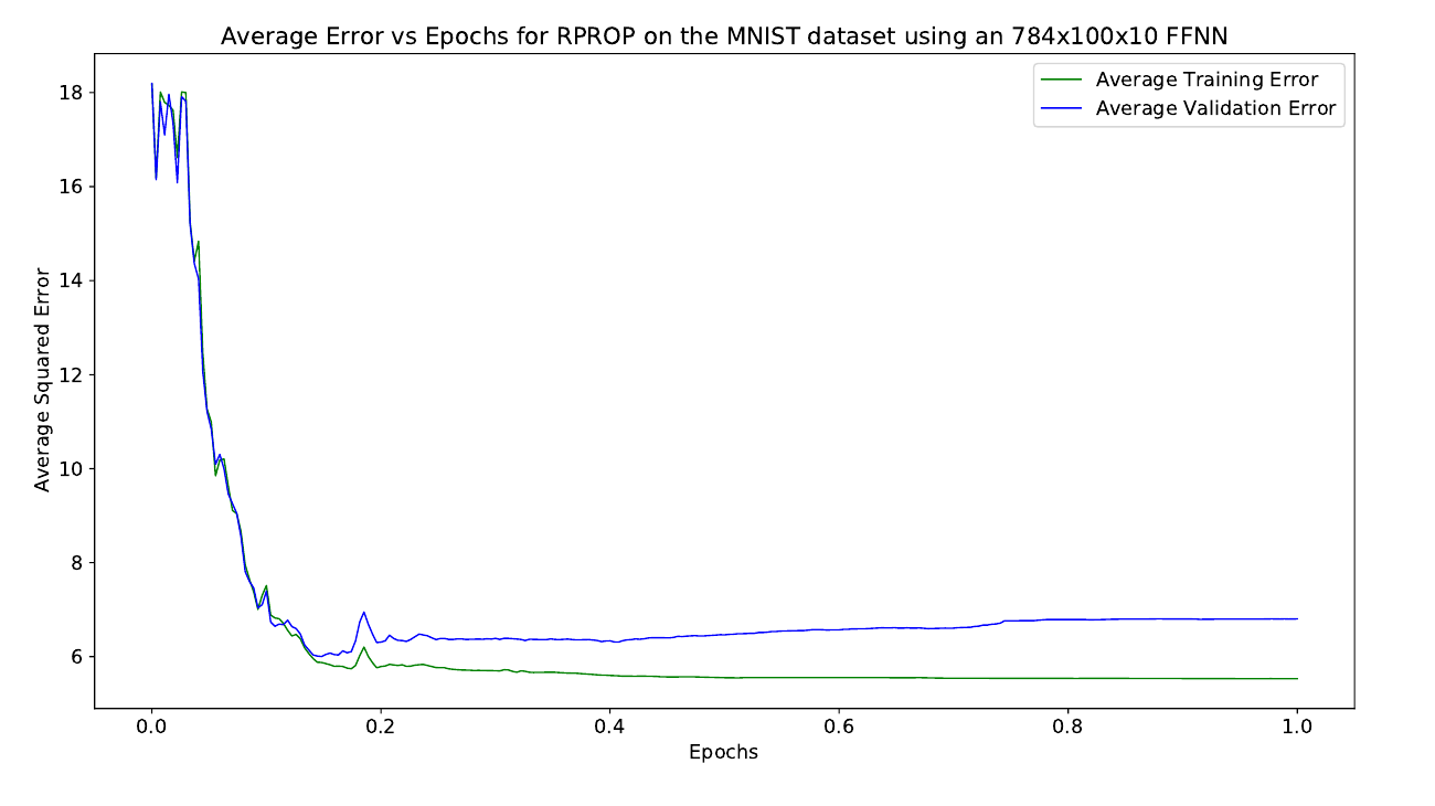
Report Figure 76, PDF p. 58 (printed p. 56). Read the x-axis: it runs from 0.0 to 1.0. This is the entire training run: one epoch.
The y-axis decodes too. The report measures error with Proben1’s squared error percentage (§11, Eqn. 11.1),
and the MNIST driver feeds it the thresholded one-hot output rather than the raw
activations (RPROPMnist.py:80,101), so every misclassified digit contributes exactly 2
and every correct one contributes 0. With outputs, that makes
So the curve starting at 18 is a network guessing at chance, and the curve flattening at 6.8 is a network at 66% validation accuracy. 70.19% on the test set is right where that plot ends. Everything is consistent; there is just far less of it than there should be.
Why it stopped
PQ (Prechelt, Early stopping: but when?) compares generalisation loss against
training progress. Both are measured over a strip of epochs, and the report’s own §11
says so: “We define a window of epochs, which are used to calculate the training
progress.” Here is the code that sets , RPROPMnist.py:41–43:
minibatchSize=min(maxBatchSize,int(np.ceil(d.TrainCount/IdealFracMinibatch)))
invTrueFracMiniBatch=1.0/np.ceil(d.TrainCount/minibatchSize)
stopStripLen=int(0.5/(invTrueFracMiniBatch*5.0))
With 54,000 training images and maxBatchSize=200, invTrueFracMiniBatch is
(one mini-batch is of an epoch), and
Twenty-seven mini-batch evaluations. A tenth of one epoch. To be the five epochs the report describes it would have had to be ; the expression is short by a factor of fifty.
And the errors it fills that strip with are recorded after every mini-batch
(RPROPMnist.py:101–104), not once an epoch, so the progress term
is measuring how much the training error moved over 27 consecutive mini-batches. Once the curve is anywhere near flat, that is a very small number, and the criterion fires when the generalisation loss exceeds with . A near-zero denominator is a criterion that fires on the first upward flicker of the validation error.
The last piece is what firing does (RPROPMnist.py:117–122): it sets epochCount=epoch,
which is the loop bound, not a break. So the current epoch still runs to completion and
then the while epoch < epochCount test fails. Fire anywhere inside epoch 0 and you get
exactly one epoch of training and exactly 271 recorded points, which, plotted against
np.arange(len(AvgTrErrors))*invMiniBatchSize (Classes/DataReporterMNIST.py:30), is an
x-axis running 0.0 to 1.0.
I re-ran it
The trained weights were never committed: Classes/DataReporterMNIST.py:18 writes them
into an Outputs/ directory that is not in the repo, and EvaluateMNIST.py:9 cheerfully
loads a file nobody else has. So the only way to check any of this was to train it again.
Everything needed is present: the MNIST idx files are committed in the sibling repo, and
the network is 400 lines of NumPy.
I ported RPROPMnist.py, Classes/MnistReader.py, the sigmoid layers of
Classes/NeuralNetworkClass.py and iRProp_plus_Layer.backwardPropagate line for line:
same weight initialisation, same initial steps, same mini-batch order,
same per-mini-batch evaluation of PQ, and ran it.
Which is a problem for the story I set out to write, because 89.76% is not 70.19%. It is within a rounding error of the naive Bayes classifier’s 89.97%.
So I took the criterion out and let the identical configuration run for sixty epochs instead of one:
The early stopping cost nothing. It stopped a run that had already stopped.
What was actually capping it
RPROP is a batch algorithm. Its entire mechanism is the ratchet on the sign of from one update to the next: agree, and the per-weight step grows by ; disagree, and it is halved. That bet only pays off if the sign is a property of the error surface. Estimate the gradient from 200 randomly chosen digits instead of all 54,000 and the sign of a small weight’s gradient is close to a coin flip, so the ratchet spends its life multiplying by 0.5, every step collapses toward zero, and the network freezes. Two flat lines from epoch 8 to epoch 60 is what that looks like from the outside. So, I suspect, is the dead-flat right-hand two-thirds of Figure 76.
Change nothing but the batch size:
| Run | Batch | Updates / epoch | Best epoch | Test accuracy |
|---|---|---|---|---|
| As written, PQ₀.₆ stops it | 200 | 270 | 1.00 | 89.76% |
| As written, PQ removed, 60 epochs | 200 | 270 | 8 | 89.53% |
| Larger mini-batch, 150 epochs | 5,400 | 10 | 140 | 95.30% |
| Full batch, 800 epochs | 54,000 | 1 | 96 | 96.26% |
Same 784×100×10 network, same iRPROP+, same data, same 90/10 split, same best-on-validation rule. The optimiser was fine; it was being asked to do something it is not for.
Two more things the re-implementation turned up
The MNIST run is not iRPROP+. It uses Classes/RPROPLayer.py, a per-layer copy of the
optimiser rather than the Classes/RPROP.py classes the Proben1 experiments use. What
distinguishes iRPROP+ from iRPROP− is one comparison: on a sign flip, revert the weight
if the error got worse. Here is the line, RPROPLayer.py:37:
self.delta_W=np.where(prevLessZero, self.delta_W if self.currentErr>self.prevErr else 0, np.sign(dE_dw_t)*self.delta)self.currentErr and self.prevErr are set to 0 in __init__ (lines 20–21) and are
never assigned again anywhere in the class: the methods that would have kept them in sync
are the commented-out block at the bottom of the file. So self.currentErr > self.prevErr
is 0 > 0, permanently false, and the flipped branch is a constant 0: the weight does
not move this iteration, its step has been halved, and its stored gradient has been zeroed.
That is precisely iRPROP−. The label on my own Figure 76 says RPROP; the driver imports
iRProp_plus_Layer; the algorithm that actually ran is iRPROP−, and I did not notice for
eight years.
It is a benign bug in the sense that iRPROP− is a perfectly good optimiser, and on the Proben1 panels it is the first of the four to reach its floor. It is not benign in the sense that the plot in my own report says one thing while my own code does another.
The learning rate is theatre. RPROPMnist.py:94 sets learningRate=10 inside the
epoch loop and passes it down through NeuralNetwork.backwardPropagate, which passes it to
each layer’s backwardPropagate. iRProp_plus_Layer.backwardPropagate accepts the
argument and never reads it, as it should, because throwing the learning rate away is the
whole idea of RPROP. But the constant sits there in the driver looking like a
hyperparameter I chose.
The sign bug in the + variants’ backtracking is a separate matter and I have written it
up in the RPROP post; it is in this file too, at the same line, and
the dead error comparison here means it can never be reached.
Draw a digit
Both models below are mine, trained in 2026: the full-batch run at the bottom of that table, and the one-epoch PQ₀.₆ run at the top of it. Same architecture, same optimiser, same data. The only difference is how long they were allowed to look at it.
With JavaScript on, this is a 280 × 280 pad you draw a digit on. The drawing is put through MNIST’s own normalisation and fed to two 784 × 100 × 10 networks at once, one trained to convergence, one stopped after a single epoch by the PQ₀.₆ criterion, with their ten output activations shown side by side and a badge when they disagree.
The normalisation matters more than the network does, and it is where most drawing demos go wrong. MNIST digits are not photographs of handwriting scaled to 28 × 28. Every one of them was cropped to the ink’s bounding box, scaled so the longer side is 20 pixels with the aspect ratio preserved, and then translated so that the centre of mass of the ink sits at the centre of a 28 × 28 field. A network trained on that has never seen a digit that fills the frame, or one that sits in a corner. Squash a 280 × 280 canvas straight down to 28 × 28 and you hand it something out of distribution and then blame the network. Untick “MNIST centring” in the widget and watch both models fall over at once.
The hidden-unit strip under the bar charts is the 100 sigmoid activations of the full run. Most of them sit near 0 or 1 for any given digit; the network is using far fewer of them than it has.
Watch the criterion fire
This is the one I wanted in 2018 and did not build. It runs the same iRPROP+ in your
browser (the Rust port compiled to WebAssembly, in a Web Worker) over 3,000 MNIST images
shipped with the post, and evaluates PQ after every mini-batch in exactly the
place RPROPMnist.py evaluates it. The one thing it does not do is obey it. It draws a
line where the criterion fired and keeps training, so you can see what got thrown away.
With JavaScript on, this trains a 784 × N × 10 network with iRPROP+ on a 3,000-image MNIST subset in a Web Worker, plots the training and validation curves live, and marks the epoch at which the PQα criterion would have stopped it, with α and the strip length k as controls.
Three things to do in it. Leave the strip at “27 updates (as run)” and watch the marker land inside the first epoch or two, then switch it to “5 epochs (Prechelt)” and watch it walk off the end of the plot: same run, same α, same curve, a criterion that now waits. Turn the mini-batch up to the full 2,700 and watch the curve stop plateauing. And switch the update rule from iRPROP+ to “as shipped” to run the optimiser the 2018 code actually ran; on this problem you will struggle to tell them apart, which is the honest reason the bug survived.
The conclusion the report reached, which still stands
The report’s comparison was fair, even though the network was crippled. A naive Bayes classifier over eight hand-designed shape features (arc length, the minimum-area box, contour count, enclosed area, Hough line counts, Harris corners) plus image moments and a 48-dimensional HOG descriptor, beat a generic 784×100×10 network trained by the best general-purpose optimiser in an eleven-way study. It was faster to train, it had no hyperparameters to get wrong, and its errors were evenly spread.
That is a real result, and the reason is not really about neural networks at all. Every one of those features encodes something a human knows about digits: that they are strokes, that holes matter, that orientation histograms are informative and absolute pixel positions are not. The 784-input network is told none of it and has to find all of it, from 54,000 examples, through a sigmoid, with a sum-of-squares loss. Give it that budget and it will lose to somebody who did the thinking in advance. The lesson generalises further than 2018: convolutions won not because they are deep but because they are the same kind of prior, written into the architecture instead of into a feature list.
The naive Bayes side of it (the features, why they work, and why the counts are initialised to one) is its own post, and it deserves the win.
But the number in this post’s title was never a fair fight, and I did not know that when I wrote the report. The thing I would tell 2018 me is not “use a CNN”. It is: your stopping criterion is a hyperparameter. It has a scale, it has units, and if you compute those units from a mini-batch count rather than an epoch count you will get a number fifty times too small and a run fifty times too short, and nothing anywhere will warn you: the loss went down, the plot has two lines on it, the pipeline produced a confusion matrix. The only evidence that anything was wrong was on the x-axis, in the figure, in the report, for anyone who looked.