Blog · Structured light ·
Scan a real object in your browser: the whole rig, start to finish
Print a board, point a projector and a webcam at a thing, and follow seven steps to a downloaded point cloud. Six posts of this series wired into one page, plus the two pieces that were missing: the local homography that turns a projector into a second camera, and guidance that tells you where to hold the board next.
- Interactive
- structured-light
- computer-vision
- camera-calibration
- point-cloud
- octree
- wasm
- webgl
Every post in this series so far has been one piece of a scanner held up on its own. Gray code labels the projector’s columns. The rig photographs the labels. The classifier decides which of them the camera actually saw. The sine rule turns a pair of rays into a point. A detector finds a calibration board and a bundle refinement turns a pile of its corners into a camera. An octree squeezes the result.
Seven working pieces, no scanner. This post is the wiring. It is one page you can open with a projector, a webcam and a sheet of A4, and follow from nothing to a point cloud on your disk. Almost none of the code below is new, and that is the point: the interesting work in a project like this is mostly composition, and the composition is where the surprises are.
Two of the pieces genuinely are new, and they are the two I like best. One is the trick that lets you calibrate a projector, which cannot photograph anything, by borrowing the decode you already did. The other is guidance: not a heat-map of where your calibration board has been, but a sentence telling you where to put it next.
What you need, and what happens if you have none of it
The real thing needs a projector (a second screen or a TV will do) and a camera pointed at the scene from beside it. A laptop’s built-in webcam faces the wrong way and cannot be used: it is looking at you, not at the object. A phone as the camera and the laptop as the projector is the combination that actually works, and it is the one post 49 is built around.
If you have none of that, everything still runs. Step 3 ships a capture bundle, step 4 ships
sixteen board views, and steps 5, 6 and 7 work on whatever step 3 decoded. You can reach a
downloaded .ply without owning a projector.
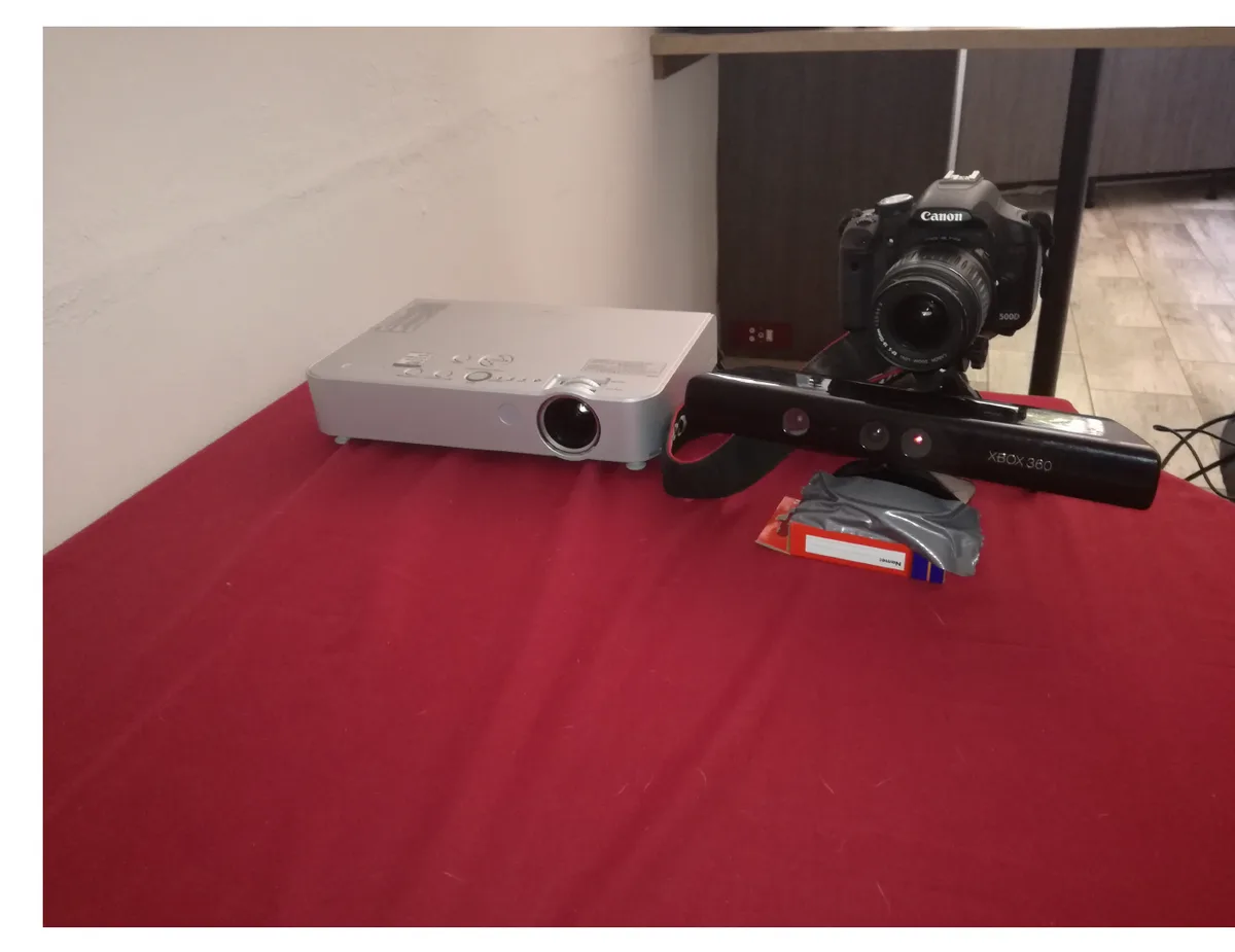
The rig this page is a browser copy of: Panasonic PT-LB51 projector, Canon 500D, and a Kinect carried along for comparison. Report Fig. 2, p. 7, and the same photograph post 49 uses.
Step 1: print the board
CameraCalibration/BoardInfo.py is nine lines of arithmetic that decide the geometry of
everything downstream: A4, blocks of 20 mm, ArUco markers of 14 mm inside the white ones, which
divides into 10 by 14 blocks and so 9 by 13 interior corners.
dpmm = 40
A4_shape = 210, 280
desired_block_size_mm = 20
desired_aurco_size_mm = 14

blocksx = A4_shape[0]//desired_block_size_mm
blocksy = A4_shape[1]//desired_block_size_mm

aurcoDict = aruco.getPredefinedDictionary(aruco.DICT_4X4_250)
charucoBoard = aruco.CharucoBoard_create(blocksx, blocksy,
                                         desired_block_size_mm,
                                         desired_aurco_size_mm,
                                         aurcoDict)
The board is the only object in the whole pipeline whose size is known, so the number you type below is the number every millimetre the scanner ever reports is scaled by. Printers routinely land a percent or two out. Measure a block.
With JavaScript on, this is the printable board, its real geometry, and a field for the block size you actually measured, which the rest of the page scales by.
Step 2: put the two devices somewhere sensible
Report §4.1 describes the placement in one sentence: the projector goes perpendicular to the scan area, and the camera sits about 25 cm to its left. The recovered translation between them, mm, confirms it: 264 mm of baseline, most of it sideways.
That number is a trade, and it is worth seeing it as one. The camera and the projector and the object make a triangle. The angle at the object, , is what converts an error in the correspondence into an error in depth, by the sine rule post 52 derives:
Push the camera close to the projector and collapses; in the denominator sends the depth error up with it, and eventually a one-pixel misread moves the answer by more than the object is big. Push it far away and is comfortable, but now the object throws a wide shadow that the projector cannot reach into, and the classifier will honestly refuse to guess in all of it. The planner below draws both.
With JavaScript on, this is a plan view of the camera, the projector and the object, with the triangulation angle and the shadow drawn, and sliders for the baseline and the distance.
The other thing report §4.1 mentions is the focus trick, and it is the sort of detail that only
shows up when you have actually done this: project a crosshair, focus the camera on the middle
of it, and both devices are now sharp on the same plane. CaptureImages/DrawCorsshairs.py
draws it, and the projector pane below still shows it first. It also still contains the bug I
found when I transliterated it for post 49, and I have kept that too, because reproducing what
the code renders rather than what it looks like it meant is the honest option.
Step 3: project, photograph, decode
The sequence is 42 frames for a 1024-wide projector: an all-black frame, an all-white one, then ten bit planes of horizontal Gray code, ten inverses, ten vertical, ten inverses. Every frame carries a small marker in its bottom-left corner spelling out its own index, with a black and a white reference cell in front so the camera can threshold itself against whatever exposure it has. That is how two devices with no channel between them stay in step, and it is post 49’s idea, not this post’s.
Then the decode, which is post 51 unchanged: Nayar’s direct/global separation off the finest bit planes, Xu and Aliaga’s five-rule classifier with and , and Eq. 4.2’s cascading XOR back from Gray to binary. The output is the thing the rest of the page is built on: for every camera pixel, which projector column and row lit it, and a flag saying when the classifier would rather not say.
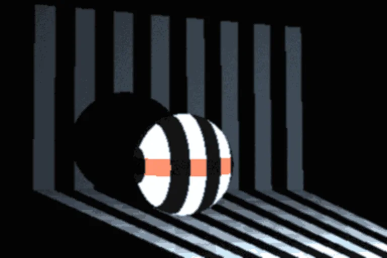
With JavaScript on, this is a full-screen Gray-code projector, a camera pane that auto-captures each frame as the marker changes, and a decoder that turns the result into a correspondence map the rest of the page uses.
Whatever you decode there is what the rest of this page works on. The strip at the top of every step says what it is currently holding.
Step 4: calibrate the camera, and be told where to put the board
This is post 61’s Levenberg-Marquardt bundle refinement
doing the work: five intrinsics, , , , and six pose numbers per view, all
minimised together against the reprojection error. CameraCalibration/main.py calls
cv2.aruco.calibrateCameraCharuco for this with
flags=cv2.CALIB_FIX_K2 + cv2.CALIB_FIX_K3 + cv2.CALIB_FIX_K4 + cv2.CALIB_FIX_K5 + cv2.CALIB_FIX_K6and report p. 11 says why in one line: “This was done as it produced the best results with the limited number of camera calibration images.” Fixing the higher radial terms to zero is not laziness, it is the right call when you have twenty-one views and a distortion model with more freedom than the data can pin down.
Which brings up the actual problem with calibrating a camera, and the thing the owner of this site asked for when he asked for this post. It is not that you need more views. It is that you need different ones. Twenty fronto-parallel boards at the same distance leave focal length and distance trading off against each other, and no number of extra views of the same pose separates them. Post 61 draws a heat-map of where your corners have landed and leaves you to work out what to do about it. That is passive.
So the widget below goes one step further and says where to hold the board next. It describes each view by four numbers a person can act on: where in the frame it sits, how much of the frame it fills, and which way and how hard it leans. Lean is read straight off the corner grid with no calibration needed, because a plane seen at an angle has its far edge shorter than its near one, so the log ratio of opposite edge lengths is a signed measure of tilt about each axis. Then it picks the emptiest bucket and tells you.
The crude version of that idea is still worth a lot. The clearest way to see it is to race a guided ordering of the same sixteen views against their file order, and watch how many views each one needs before the focal length settles.
With JavaScript on, this adds calibration views one at a time, re-fits the whole bundle after each, draws where each board landed in the frame, and tells you where to hold it next. It also races a guided ordering of the same views against their file order.
Step 5: calibrate the projector, which cannot see
Here is the problem that makes this repo interesting. A projector is a camera run backwards: it has a focal length, a principal point, and lens distortion, and reconstruction needs all of them. But you calibrate a camera by photographing a board with it, and a projector cannot photograph anything. It has no corners of its own.
Report §4.2.3 takes Moreno and Taubin’s answer. Project the Gray code onto the board while it is being photographed, decode it, and now every camera pixel carries the projector pixel that lit it. The corner the detector found at camera pixel has a projector coordinate too. Look it up.
Except you cannot just look it up, and report p. 11 says exactly why:
it is inaccurate to directly transform the corners of the checkerboard from the camera’s frame of reference to the projectors as the position is only accurate up to the nearest pixel.
Two things are wrong with a direct lookup. The corner is sub-pixel, found to a fraction of a camera pixel by the saddle refinement, and a lookup rounds it to a whole one. And the decoded value itself is an integer projector index, quantised by construction, with noise on top. You have thrown away most of the precision you spent the whole detector earning.
Moreno and Taubin’s fix is the local homography. Over a small patch, the board is a plane, and a plane maps to a plane through a :
So gather every trusted correspondence in a patch around the corner, fit one to
the lot, and push the corner’s exact sub-pixel position through it. Hundreds of noisy integer
readings average into one sub-pixel answer. GetSecondViewPoints.py is the whole idea in
about twenty lines:
indices = np.indices((47, 47)).reshape(2, -1).T - 23

for pt in charucoCorners:
    surroundingPoints = (np.rint(pt[:]) + indices).astype(np.int32)
    # ... clip to the image ...
    isValid = np.logical_and(validV[surroundingPoints[:, 0], surroundingPoints[:, 1]] == 0,
                             validH[surroundingPoints[:, 0], surroundingPoints[:, 1]] == 0)
    surroundingPoints = surroundingPoints[isValid]
    projector_points_u = coordsV[surroundingPoints[:, 0], surroundingPoints[:, 1]]
    projector_points_v = coordsH[surroundingPoints[:, 0], surroundingPoints[:, 1]]

    if len(projector_points_v) > 0 and len(projector_points_u) > 0:
        projector_points = np.stack((projector_points_u, projector_points_v), axis=1)
        surroundingPoints[:, [0, 1]] = surroundingPoints[:, [1, 0]]
        H, mask = cv2.findHomography(surroundingPoints, projector_points,
                                     ransacReprojThreshold=2, maxIters=100000,
                                     method=cv2.FM_LMEDS, confidence=0.99)
        pt2 = np.dot(H, [pt[0, 1], pt[0, 0], 1.0])
        pt2 /= pt2[2]
A 47 by 47 patch, masked against the classifier’s own two invalid maps so no pixel it refused to commit on gets a vote, and one robust homography per corner.
The decode is what makes calibrating the projector possible at all. That is the dependency I find loveliest in this whole repository. The Gray code exists so the reconstruction can find correspondences; it turns out to be the only reason the reconstruction has a calibrated projector to reconstruct with.
The widget below is that fit, live. Click anywhere on the decoded scene and it gathers the patch, throws away the pixels the classifier flagged, runs the same least-median-of-squares search, and shows you the two answers side by side: the nearest whole decoded projector pixel, and the sub-pixel one the homography gives. Because the bundled sample recorded the rig that rendered it, it can also tell you the true answer, and how far each one is from it.
On the bundled sample, clicking the ball at camera pixel gives the flavour of it. The decoded correspondence there is projector pixel , which is 0.42 px from where that point really projects, because rounding to a whole pixel is the best a lookup can do. The local homography, fitted to the 441 correspondences in a 21 by 21 patch around it, says : 0.09 px out. That factor of four or five is what a whole calibration is then built on, and the real thing has it easier still, because it does this on a flat board where the plane assumption is exact rather than on the side of a sphere.
Turn least median of squares off and you get a plain least-squares fit over every pixel in the patch, including the ones sitting on a depth discontinuity where the plane assumption is simply false. The difference is the whole reason for the robust estimator.
With JavaScript on, this lets you click a pixel of the decoded scene, fits a local homography to the patch of correspondences around it, and compares the sub-pixel projector coordinate it recovers against the nearest whole decoded pixel.
Once the projector has corners it has a calibration, fitted with exactly the same machinery as
the camera’s, on exactly the same board points. And that leaves the last unknown: where the two
devices are relative to each other. Each board view gives the board’s pose in the camera and
the same board’s pose in the projector, so composing one with the inverse of the other gives
the rigid transform between them, once per view. main.py hands that job to OpenCV:
retval, cameraMatrix1, distCoeffs1, cameraMatrix2, distCoeffs2, R, T, E, F = \
    cv2.stereoCalibrate(all_real_points, all_charco_corners_camera_2, all_charco_corners_projector,
                        mtx_camera, dist_camera, mtx_proj,
                        dist_proj, camera_resolution, flags=cv2.CALIB_FIX_INTRINSIC)
CALIB_FIX_INTRINSIC says: both cameras are already calibrated, only solve for the pose. What
stereoCalibrate does first is precisely that per-view composition, averaged; then it refines
everything jointly. The widget above does the first half over the real per-view poses your step
4 fit produced, and reports the spread across views, which is the number that tells you whether
the average means anything. It does not do the joint refinement, and I have not pretended it
does.
That out of 768 is worth a second look: the projector’s principal point sits nowhere near the middle of its image. That is not an error, it is lens shift. A projector on a table throws its image upwards so the picture lands on the wall rather than the floor, and its optical axis leaves through the bottom of the frame. A model that assumed a centred principal point would be wrong by 300 px here.
Step 6: two rays, a baseline, a triangle
Post 52 has the derivation. Back-project the camera pixel and
the projector pixel to rays, take the angle at each end of the baseline, and the third angle
follows from ; then the sine rule gives the distance along the
camera ray. No least-squares midpoint, no cv2.triangulatePoints, one triangle per pixel,
vectorised over about ten million of them in the original.
The one addition my Rust port makes is a refusal. As the object recedes, and , and in the denominator amplifies whatever floating-point noise is left into a wild depth. A plain implementation returns a huge or negative or NaN there instead of admitting it does not know, so the port rejects the pair below a minimum and says how many it rejected.
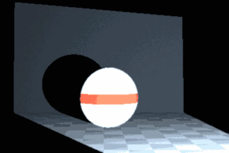
The fully-lit frame of the bundled sample. The black surround is not darkness, it is everywhere the projector’s cone does not reach: its field of view is genuinely narrower than the camera’s. The hard-edged disc on the wall is the ball’s own shadow, and the classifier will decline to decode inside it, correctly.
With JavaScript on, this triangulates every trusted correspondence into a coloured point cloud you can orbit, voxel-downsamples it, and downloads it as a .ply that MeshLab or CloudCompare will open.
Step 7: throw most of it away
A dense scan is a list of positions, and most of those positions are near-duplicates of a
neighbour, quantised at a precision the scanner never had. Post 64’s
octree keeps the occupancy instead: which cell of a repeatedly-subdivided cube has anything in
it. The saving is structural rather than clever, because the Morton code of a cell is its
coordinate, so once you have stored the code you do not store a position at all. Four bytes of
code and three of colour per occupied leaf, against the roughly forty bytes an ASCII .ply
spends writing three floats and three integers as text.
Report §6.6 measured the same thing on the real scans, at 1 mm resolution:
| Scene | Point cloud | Octree |
|---|---|---|
| Cup | 4716 KB | 164 KB |
| Dragon Party | 6238 KB | 162 KB |
| Statue | 10513 KB | 84 KB |
| Toy Car | 7891 KB | 176 KB |
The statue is the interesting row: the largest cloud and the smallest octree, because a statue is a single dense surface at close range and its points pile many-to-one into the same cells.
On the bundled sample the same thing happens at a smaller scale. At depth 7 over a 583 mm cube,
so 4.55 mm cells, 58,005 points land in 17,018 occupied cells out of the 2,097,152 a dense
grid at that depth would need, which is 0.81% of them. The file is 116 KB against the
.ply’s 2,092 KB, eighteen times smaller, and the only thing lost is a resolution the
scanner never had.
With JavaScript on, this builds the octree over the cloud from step 6 at a depth you choose, shows how few of the cells are occupied, and downloads it as a small binary file.
What this cost, and what it did not
Seven steps, and six of them are other posts’ code called with different arguments. The honest inventory:
| Step | Where it comes from | New here |
|---|---|---|
| Board and detector | post 60, calib-wasm | nothing |
| Projector pane, sync marker, bundle format | post 49 | promoted to a shared module |
| Decode | post 51, graycode-wasm | nothing |
| Bundle refinement | post 61, calib-wasm | the guidance around it |
| Local homography | this post | all of it |
| Stereo pose | this post | the composition, not the joint refinement |
Triangulation and .ply | post 52, graycode-wasm | nothing |
| Octree | post 64 | the binary file format |
The two new pieces are about four hundred lines between them, and the local homography is the one that matters. It is also, oddly, the piece that most repays being pulled out of a twenty-line numpy function and looked at: fitting a plane-to-plane map over a neighbourhood to recover a sub-pixel value from quantised integer readings is a trick that has nothing to do with projectors, and it works anywhere you have a dense, noisy, integer-valued correspondence field and want one precise value out of it.
The reduction I made is in step 5. A full projector calibration wants a set of board views each
captured under the full Gray-code stack, which is forty-two photographs per pose and
twenty-one poses, and no such set exists in the repository or would be reasonable to ship. So
step 5 fits the local homography on real decoded data, which is the interesting half, and takes
its projector intrinsics either from the bundle’s own metadata or from the report’s published
matrices, rather than re-deriving them from board captures that do not exist. The pose
composition runs on your real per-view camera poses; the joint refinement stereoCalibrate
does after it is not reproduced.
That is the series. It started with a projector painting numbers onto a wall and ends with a file on your disk, and the only thing between them is arithmetic anyone can follow.