Blog · Bayesian filtering ·
EKF-SLAM: one covariance matrix for the robot and everything it has ever seen
The pose and every landmark in one state vector with one joint covariance, ported from a C++/Eigen RGB-D system to a room you can drive a robot around, with the covariance matrix drawn live, so the off-diagonal blocks that make SLAM work are finally visible.
- Interactive
- slam
- ekf
- kalman-filter
- state-estimation
- bayesian-filtering
- rgb-d
- c++
SLAM is a chicken-and-egg problem. To know where the robot is you need a map to place it in; to build the map you need to know where the robot was when it looked. Neither half can be solved first.
EKF-SLAM’s answer is blunt and, once you see it, rather beautiful: stop treating them as two problems. Put the robot’s pose and the position of every landmark it has ever seen into one state vector, keep one joint covariance matrix over all of it, and run the Extended Kalman Filter from three posts ago on the whole thing. The map and the pose then correct each other through the off-diagonal blocks of that matrix (the robot–landmark and landmark–landmark correlations), which is the part of the machinery nobody ever draws. This post draws it.
The system this comes from was written in C++ with Eigen and OpenCV, in November 2018 (the source headers say “Created on: 03 Nov 2018”), for a 6-DoF camera pose and 3-D landmarks found with SURF, and run over RGB-D sequences from the TUM Freiburg1 benchmark. This is what it produced on the desk sequence, the reconstruction rendered from its own estimated trajectory:
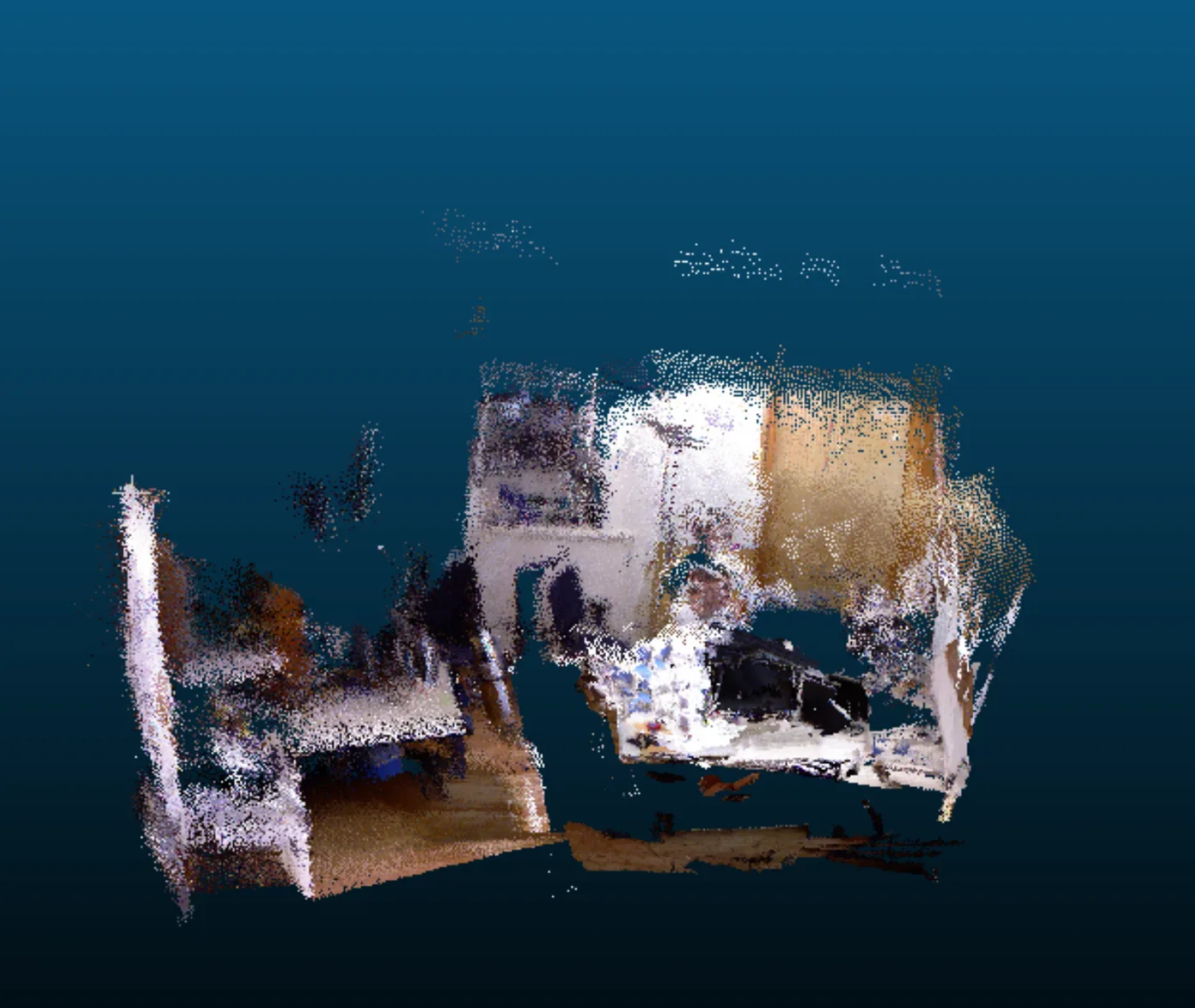
The Freiburg1 desk scene, reconstructed by placing every depth frame on the pose the
EKF-SLAM estimated for it. (docs/pngs/res.png in the repo.)
None of that runs in a browser: ROS, rosbag, PCL, OpenCV-contrib and half a gigabyte of bags per sequence. What does run is the same filter, reduced to two dimensions, in a room where you are the robot. That is the widget further down, and it is honestly the better teaching artefact. But first the machine, as built.
The pipeline
Figure 1 of the report is the whole algorithm as a flowchart, and it is worth tracing before any equation, because two of the boxes (Matrix Extraction and Diverged?) are where the engineering lives.
Figure 1 of the report, page 5, redrawn. One frame goes round the loop once. A frame without enough matches is skipped; a frame whose refinement diverges is thrown away whole; only a converged frame is allowed to add new landmarks.
Read it as: see, match, predict, extract, refine, check, grow. Each frame’s SURF features are matched against every descriptor the map has ever stored (that is what makes relocalisation possible after getting lost, and it is also what §6 later blames for the map’s decline). If enough matches survive, the filter predicts, pulls only the relevant rows and columns of the joint covariance out into a small matrix, runs an iterated correction on that, and either commits the result and admits new landmarks or discards the entire frame.
One state vector, one covariance
Eq. (2.11) of the report writes the state as the camera’s six degrees of freedom followed by three numbers per landmark:
with ZYX Euler angles. The report spends a paragraph on why Euler angles and not a rotation matrix or Rodrigues: a matrix is nine numbers for a three-degree-of-freedom quantity and the filter would happily drift it off the set of valid rotations, and with Rodrigues the Jacobian about an arbitrary current rotation is awkward. I still think that was the right call for a first implementation, even though the rotational error is exactly where this system loses to the published ones.
The joint covariance is with . The code keeps it in pieces:
PosStateVariance (), LandMarkStateVariance (up to
MAX_LANDMARK_SIZE MAX_LANDMARK_SIZE) and two cross blocks,
PosLandMarkRowStateVariance and PosLandMarkColStateVariance. But it is one matrix,
and the cross blocks are the ones this post is about.
In the widget the pose is and a landmark is , so ; with twenty landmarks that is a matrix, small enough to draw cell by cell.
The motion model is the identity
The first engineering decision, page 8 of the report. A constant-velocity model was tried (it adds six velocity states and predicts the camera onward each frame), and it made things worse on the RGB-D sequences. The motion of a hand-held camera is stochastic, and a prediction in the wrong direction on a frame that then fails to match anything is not corrected; it compounds, and the next frame matches even less. So became the identity and the entire burden moved to the correction step:
which is why PredictionStep, EKFSlam.cpp lines 234–238, is the shortest function in
the file:
void EKFSlam::PredictionStep(double deltaTime){
	double dt_sq = (deltaTime*deltaTime);
	this->PosStateVariance += this->Q*dt_sq;
	this->max_squared_dist_to_travel += dt_sq*DELTA_DIST_THRESH_SQ;
}
Only the pose block of grows. Landmarks do not move, so their rows of are zero and an unobserved landmark’s uncertainty is frozen until it is seen again.
Where comes from is the part I like. Rather than tune six variances by hand, the report starts from a physical limit: the fastest the camera plausibly moves, read off the ground truth, is about . Take that to be the point of the per-frame displacement, and
with the assumed rotational limit. The widget does exactly this in 2-D from the robot’s own limits ( and ) at twenty steps a second; the “assumed top speed” slider is , and is derived from it every step rather than set.
The observation, and its Jacobian
The sensor is a depth camera, so a matched feature comes with a 3-D position in the camera’s frame. Eq. (2.18) writes what the filter expects to see for a landmark from a pose with translation and rotation :
The report considered converting this to range and bearing and chose not to: the Cartesian form is the simplest, and its Jacobian comes apart by inspection. , , and the derivative with respect to the three angles is assembled from three matrices, one per angle, weighted by the offset to the landmark (Eq. 2.20):
where , , (Eqs 2.21–2.23) are the
element-wise derivatives of ‘s columns, written out in full in
GetJRxyz, lines 80–88. I will spare you the nine-term trigonometric entries; the point
is that they are constant for a frame and the per-landmark Jacobian is three of them
scaled and summed. Stacked, one row-block per observed landmark, Eq. (2.24) is very
sparse:
Every row-block touches the pose columns; each touches exactly one landmark’s columns. That shape is what makes the extraction step in the next section legitimate.
In two dimensions all of this collapses to one angle. With and , the widget’s row-block for landmark is
and the middle column is with only one term left in it.
Where (the measurement noise) comes from is less principled, and the
report says so. reprojectPointWithSigmaInterval, lines 100–114, back-projects the pixel
at its depth and again at depth plus one raw unit, and calls half the difference a
standard deviation:
void EKFSlam::reprojectPointWithSigmaInterval(double depth, const cv::Point2f &pt, Eigen::Vector3d &pt3d, Eigen::Vector3d &var3d){
	double Z = depth / SCALING_FACTOR;
	double Zp1 = (depth + 1.0) / SCALING_FACTOR;

	double n_x = (pt.x-CAMERA_C_X)/ CAMERA_FOCAL_LENGTH;
	double n_y = (pt.y-CAMERA_C_Y)/ CAMERA_FOCAL_LENGTH;
	double X = n_x*Z;
	double Y = n_y*Z;

	double sigma_x = std::abs(n_x*Zp1-X)/2.0;
	double sigma_y = std::abs(n_y*Zp1-Y)/2.0;
	double sigma_z = std::abs(Zp1-Z)/2.0;
	pt3d << X, Y, Z;
	var3d << sigma_x*sigma_x, sigma_y*sigma_y, sigma_z*sigma_z;
}
One raw depth unit is m, so this gives a of a tenth of a millimetre:
a “2σ interval” on the quantisation of the depth image and nothing else. Page 9 admits
that it ignores pixel quantisation entirely and that a mis-matched feature with a variance
that small drags the pose after it. So getSmallerStateVectors adds a term the report
describes as “experimentally set to times a feature’s match distance”:
line 273, match_distance[loop]*1e-1+2e-6. A worse descriptor match is a less trusted
position. In practice that term is the whole of .
The matrix-extraction step
Page 10: the matrix inversion required to calculate the Kalman gain is an expensive
operation, so the relevant matrix elements are extracted from the global matrices before
processing. The gain (Eq. 2.9) needs
, and because
has non-zero columns only for the pose and the landmarks in this frame,
that product depends only on the corresponding rows and columns of . With
landmarks matched, the matrix to invert is whatever the size of the map.
getSmallerStateVectors, lines 256–267, gathers those blocks into Pk:
	for (int loop = 0; loop < number_of_observations; loop++){
		int state_offset_obs_pt_ind = obs_pt_ind+POSITION_VECTOR_SIZE;
		int startPointInState=offset_rw_obs_ind[loop];

		Pk.block(0, state_offset_obs_pt_ind, POSITION_VECTOR_SIZE, LANDMARK_LENGTH) << this->PosLandMarkRowStateVariance.block(0,startPointInState,POSITION_VECTOR_SIZE,LANDMARK_LENGTH);
		Pk.block(state_offset_obs_pt_ind, 0,LANDMARK_LENGTH, POSITION_VECTOR_SIZE)  << this->PosLandMarkColStateVariance.block(startPointInState,0,LANDMARK_LENGTH,POSITION_VECTOR_SIZE);

		int current_i2=POSITION_VECTOR_SIZE;
		for (int loop2 = 0; loop2 < number_of_observations; loop2++){
			Pk.block(state_offset_obs_pt_ind, current_i2,LANDMARK_LENGTH,LANDMARK_LENGTH) << this->LandMarkStateVariance.block(startPointInState,offset_rw_obs_ind[loop2],LANDMARK_LENGTH,LANDMARK_LENGTH);
			current_i2+=LANDMARK_LENGTH;
		}
That is exactly right for the inversion. It is not the whole update, and here is the thing I did not see in 2018. The full correction is with , and has a non-zero row for every state that is correlated with an observed one, which after a few frames is every landmark in the map. Observing landmark 3 moves landmark 17, if the two were mapped from the same uncertain pose, and shrinks its covariance too. That is not a side effect of EKF-SLAM. It is EKF-SLAM: the mechanism by which re-seeing an old landmark tightens the whole map is precisely those rows.
UpdateStateAndVariance, lines 317–332, writes back the pose, the observed landmarks and
the blocks between them, and nothing else:
	this->PosState = StateUpdate.segment(0,POSITION_VECTOR_SIZE);
	this->PosStateVariance << VarianceUpdate.block(0, 0, POSITION_VECTOR_SIZE, POSITION_VECTOR_SIZE);
	for (int loop = 0; loop < number_of_observations; loop++){
		int state_offset_obs_pt_ind = obs_pt_ind+POSITION_VECTOR_SIZE;
		int startPointInState=offset_rw_obs_ind[loop];

		this->PosLandMarkRowStateVariance.block(0,startPointInState,POSITION_VECTOR_SIZE,LANDMARK_LENGTH) << VarianceUpdate.block(0, state_offset_obs_pt_ind, POSITION_VECTOR_SIZE, LANDMARK_LENGTH);
		this->PosLandMarkColStateVariance.block(startPointInState,0,LANDMARK_LENGTH,POSITION_VECTOR_SIZE) << VarianceUpdate.block(state_offset_obs_pt_ind, 0,LANDMARK_LENGTH, POSITION_VECTOR_SIZE);
		int current_i2=POSITION_VECTOR_SIZE;
		for (int loop2 = 0; loop2 < number_of_observations; loop2++){
			this->LandMarkStateVariance.block(startPointInState,offset_rw_obs_ind[loop2],LANDMARK_LENGTH,LANDMARK_LENGTH) << VarianceUpdate.block(state_offset_obs_pt_ind, current_i2,LANDMARK_LENGTH,LANDMARK_LENGTH);
			current_i2+=LANDMARK_LENGTH;
		}
		this->LandMarkStateVector.segment(startPointInState,3) = StateUpdate.segment(state_offset_obs_pt_ind, 3);
		obs_pt_ind+=LANDMARK_LENGTH;
}The IEKF loop and its guard rails
The correction is iterated, as in post 18: re-linearise
about the current answer, correct again, until the error stops improving. This is
processImage, lines 372–408, with the debug prints and commented-out lines removed:
	for (int iteration =0; iteration < MAX_REFINEMENT_ITERS; iteration++){
		this->recalculateRelevantV(relevantX, ObservedValues, ek, Jh);
		Eigen::MatrixXd PfJht = Pk*Jh.transpose();
		Eigen::MatrixXd mtxToInvert = Jh*PfJht + Rk;
		Eigen::MatrixXd KkT = (mtxToInvert.transpose().householderQr().solve(PfJht.transpose())).transpose();
		double solution_error = (KkT*mtxToInvert - PfJht).norm() / PfJht.norm();
		if (solution_error > 3e-4){
			return;
		}

		StateUpdate = KkT*ek;
		VarianceUpdate = (IdentityMat - (KkT*Jh))*Pk;
		relevantX += StateUpdate;
		Pk = VarianceUpdate;

		curr_err_norm = ek.norm();
		if (prev_error_norm<1.02*curr_err_norm){break;}
		prev_error_norm = curr_err_norm;
	}
	curr_err_norm /=eq_obs_size;
	if (curr_err_norm>0.05){
		std::cout << "Error too high to add new features \n\n";
		return;
	}
	double deltadist = (this->PosState.segment(0,3) - relevantX.segment(0,3)).squaredNorm();
	if (deltadist>this->max_squared_dist_to_travel){
		std::cout << "I see the machine tried to warp through space. I will not allow this. \n\n";
		return;
	}
	this->max_squared_dist_to_travel = 0;
	this->UpdateStateAndVariance(relevantX, Pk, offset_rw_obs_ind);
Four things in there I would still do today.
- No explicit inverse. The gain is found by solving
with a Householder QR, the same idea post 18 recommended over
np.linalg.inv. - Then the solve is checked.
solution_erroris the relative residual of that linear system. If it is above the frame is abandoned, because a gain that does not satisfy its own equation is a gain computed from an ill-conditioned , and that means a bad match somewhere. It costs one matrix product. - The stopping rule is a plateau, not a tolerance. The loop breaks when the previous
error is not at least 2% larger than the current one. Post 18 found that iterating the
correction to convergence runs Newton’s method on the measurement equation and forgets
the prior; stopping on a plateau after a pass or two is a pragmatic hedge against that,
and it also means the covariance (note
Pk = VarianceUpdateinside the loop, unlike the Python version, which held fixed) is only shrunk a few times. - The warp gate. After the loop, the proposed pose is compared with the previous one. If it moved further than the speed limit allows since the last accepted frame, the frame is discarded with the message quoted above. A single confidently-wrong match can move the pose by metres; the physics says that cannot have happened, so the filter is not allowed to believe it.
Data association, where SLAM actually lives
Everything above assumes each measurement arrives labelled with the landmark it belongs
to. The labelling is the hard part. The header, EKFSlam.hpp lines 15–44, is the
system’s entire tuning surface, and all of it is about that:
#define CAMERA_FOCAL_LENGTH 525
#define CAMERA_C_X 319.5
#define CAMERA_C_Y 239.5
#define SCALING_FACTOR 5000.0
#define MIN_KEYPOINTS 12

#define LANDMARK_LENGTH 3
#define POSITION_VECTOR_SIZE 6
#define MAX_LANDMARK_SIZE 30000

#define CLOSEST_MATCH_THRESH 0.15
#define CLOSEST_MATCH_THRESH_RATIO 0.68
#define MAX_MATCH_THRESH 0.24

#define MAX_LANDMARKS_IN_FRAME 40

#define CLOSEST_CANDIDATE_THRESH_FF 0.4
#define CLOSEST_CANDIDATE_THRESH 0.4
#define MIN_CANDIDATE_THRESH_FF 300
#define MIN_CANDIDATE_THRESH 250

#define CURRENT_STATE_VARIANCE_MULTIPLE_ADD 3
#define CURRENT_STATE_VARIANCE_ADDITION_ADD 2e-4

#define MAX_REFINEMENT_ITERS 10
#define DELTA_DIST_THRESH_SQ 18
SURF with the extended 128-element descriptor, brute-force matched against the whole
map’s descriptor matrix with the two nearest neighbours returned. A match is accepted
only if all three hold, DetectAndSeperateKeypoints lines 197–199:
		if (match[0].distance < MAX_MATCH_THRESH &&
			match[0].distance<match[1].distance*CLOSEST_MATCH_THRESH_RATIO &&
			match[0].distance+CLOSEST_MATCH_THRESH<match[1].distance) {
That is an absolute ceiling, Lowe’s ratio test, and an absolute gap to the runner-up. Then
a geometric sanity check that the matched landmark is roughly the right distance away
(line 184: a threshold of , loosening
as the pose becomes less certain). A feature that matches nothing well
(CLOSEST_CANDIDATE_THRESH) and has a strong detector response becomes a candidate;
after a converged frame, candidates that are also dissimilar from each other are added,
strongest response first, up to MAX_LANDMARKS_IN_FRAME minus the number matched. The
report’s reason for the cap is exactly right: a map cluttered with weak, redundant points
dilutes the certain ones.
A wrong match is worse than no match. No match costs a frame; a wrong match is a confident measurement of the wrong thing, applied through a gain that was computed believing it. That is what the report’s §6 blames for most of the system’s error, and it is why two of the four guard rails above exist.
Watch a landmark converge
Figure 36 is the report’s best conceptual figure, and it is what the widget’s ghost
trail is built to reproduce. A fork of the code (EKFSlamGenCov/) dumps the landmark
block of to CSV every frame from frame 8 to 30, and a 36-line script
eigen-decomposes one landmark’s block and draws its , and
ellipses.
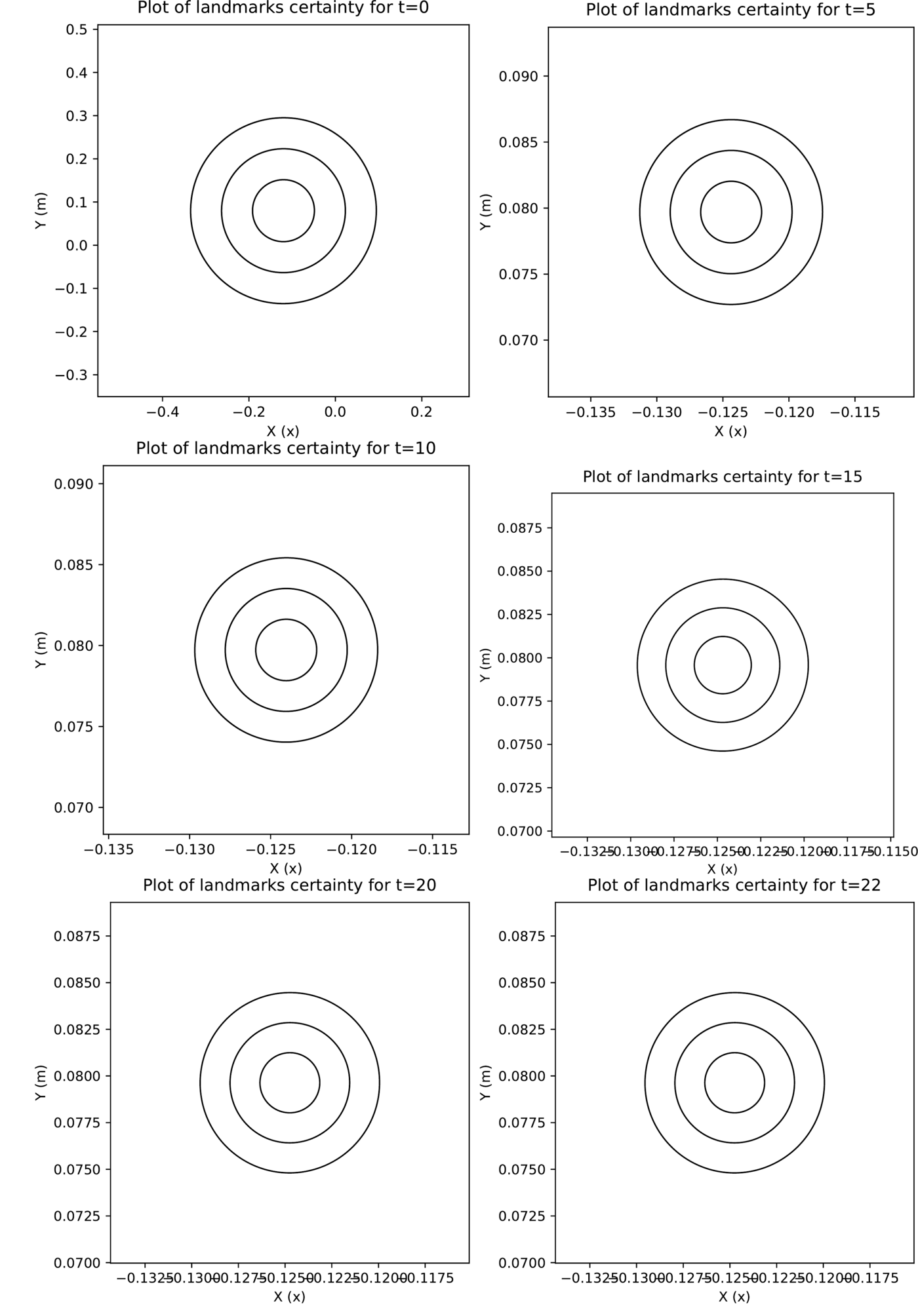
Figure 36, page 29: the , , ellipses of one landmark at . Read the axes: the first panel spans roughly m, the rest about m. By the outer ellipse is about 5 mm across and from then on it barely moves.
The shape of that curve is the running-mean law from post 17: the first observation halves the variance, the tenth removes a tenth of what is left, and the measurement noise floor is reached in a handful of frames. §6 puts the tension plainly: raise a landmark’s confidence too fast and one outlier match wrenches it; too slowly and the robot is forever navigating by landmarks it does not trust.
Play with it
A room, ten by eight metres, two dozen landmarks, and a robot with a sensor that reports the position of any landmark within its range and field of view, in its own frame, with Gaussian noise: the 2-D version of a depth camera with a perfect descriptor matcher. The filter never sees the controls; it sees measurements and ids.
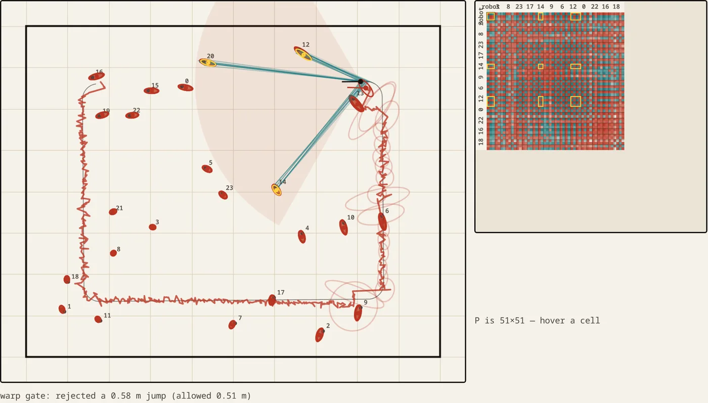
With JavaScript on, this becomes a room you can drive a robot around, with the EKF-SLAM estimate, every landmark’s ellipse, and the joint covariance matrix updating live.
Drag on the room to steer, or click it and use the arrow keys or WASD; the autopilot tours the room on a loop when you leave it alone. Things to try, roughly in order:
- Watch the robot’s ellipse breathe. It grows every step by (the identity model knows nothing) and snaps shut the moment a mapped landmark is in view. Drive into a corner facing the wall and it inflates; turn round and it collapses in one frame. That is the whole of Eqs (2.16) and (2.10) as a picture.
- Watch the ghosts. Each landmark leaves a trail of its past 95% ellipses, big and pale on first sight, then shrinking fast, then not at all: Figure 36, for every landmark at once. Switch the trail off if it gets busy.
- Watch . The heatmap is the joint covariance, log-scaled, with the robot’s block top-left and each landmark’s block down the diagonal. Everything off the diagonal is a correlation. When a landmark is first seen its row lights up against the robot block; as the robot moves on and sees others, the landmark–landmark blocks fill in too. Hover a cell to see which pair it couples and the correlation coefficient. The outlined blocks are the sub-matrix that entered this frame’s inversion: the matrix-extraction step, live.
- Close a loop. Let the autopilot run the first lap. By the time it returns to the start, the map’s far corner was built on a pose that had drifted; when it re-sees a landmark from the beginning the status line reports a loop closure and the mean landmark drops. Now switch the bookkeeping to as shipped in 2018, reset, and watch the same lap: the landmark in view tightens, the ones out of view do not, the correction never reaches the far side of the room, and in a room this sparse the map comes apart within a lap, with the error gate rejecting frame after frame. On the desk sequences, where almost every frame re-sees most of the map, the same shortcut held to a few centimetres (Table 1 below); it is the sparse, forward-looking case that exposes it.
- Lose the robot. Two seconds of no measurements: the ellipse balloons, the estimate sits still while the real robot keeps going, and the first frame back has to close the gap. With the warp gate on, that first frame is sometimes rejected as impossible (the status line says so), and the second one, with a larger allowance, is accepted.
- Mis-associate. The two mapped landmarks in view that lie closest together swap ids for a second. This is what a confused descriptor matcher does, and the response is the failure §6 describes: the map lurches, because the filter is confidently told that landmark 7 is where landmark 12 is. If the pair is far apart the warp gate catches it; if they are close, it goes straight through. Try it with the gate off.
- IEKF passes at 1 is a plain EKF, and in this world it often cannot cope: with the identity model the heading innovation each step is large, a single linearisation about the prior does not fit it within the error gate, and the readout fills with rejected frames until the pose has drifted off. Two or three passes fix it. That is page 34’s “the linear approximation holds for small rotational movements only”, live, and the reason the C++ iterates at all.
- Edit the map. Toggle Edit landmarks and click to add one, click one to remove it, or drag one to move it. The filter is not told, and you can watch a landmark’s estimate get dragged toward its new position by measurements that no longer agree with the map.
- The score at sixty seconds is the mean distance between mapped landmarks and where they really are. Different driving strategies give different scores; a slow sweep that keeps a few known landmarks in view beats a fast dash every time.
Why not WASM
With twenty landmarks the joint state has 43 entries, the matrix that is actually inverted is for landmarks in view (typically to ), and the exact update is an product. Measured in Node on the widget’s own scenario, three IEKF passes, exact mode: about 0.35 ms a frame at 20 landmarks, 0.7 ms at 30 and 5 ms at 60 (where a 120° wedge sees a dozen at a time and the inverted matrix is ); shipped mode, which never touches the rest of , is a quarter of that. In headless Chrome, with a full map and the widget’s own drawing left out of the number, it reads 0.33 ms at 20 landmarks and 5.3 ms at 60; the readout prints the live figure.
The cost of the exact update grows as , so it is the size that bites. Extrapolating, two hundred landmarks is a matrix and something like 25 ms a frame in JavaScript: the point at which a compiled kernel would start to matter, and a sentence about why rather than a build. It is also, in miniature, why the field moved on from EKF-SLAM. is dense and quadratic in the map, and for a map of thousands of features it is not the inversion that kills you but the fact that every frame touches every entry. Sparse information filters and graph-based back-ends keep the same probabilistic model and throw away the dense matrix; that is the direction the “what I’d fix” list below is pointing at.
What I’d fix
§6 of the report, page 34, rephrased and with what I think now added.
- Two descriptor sets, not one. Matching every frame against the entire map’s descriptors is what makes relocalisation possible, but the matrix grows every frame and so does the rate of false matches. Keep a recent set for tracking and fall back to the global one only when lost.
- RANSAC on the matches. Geometric outlier rejection before the filter ever sees a measurement, instead of after the fact through the warp gate.
- Loop closure and bundle adjustment. The report lists these as smoothing steps. In hindsight, the first thing to do is the exact covariance update: the loop closure the filter is supposed to give you for free was the very thing the extraction shortcut switched off.
- A coarse motion estimate before the EKF. Rotation is the weak point: Table 2 on page 33 has the EKF at 10.6° RMSE on the rotation-heavy sequence against 2.2° for ORB-SLAM2, because the first-order expansion of holds for small rotations only. Feeding the correction a rough pose from somewhere else would put the linearisation point near the answer and cut the IEKF passes.
- A particle filter for the multi-modality. When two features look alike the matcher switches between them, the posterior over that landmark is two bumps, and a Gaussian can only ever sit between them. §6 points at the particle filter from three months earlier as the tool for that job, and Table 3 of the report is a seven-row comparison of the two. The next post is the honest benchmark against RGB-D SLAM and ORB-SLAM2, and what those numbers say about all of the above.