The Kalman filter, derived by someone who had to implement it

Assignment 4 of EAI732: Intelligent Systems asked for the Kalman filter and the particle filter, from first principles, benchmarked against each other. I wrote 27 pages about it. What I remember most clearly is that the derivation only made sense to me after I had written the scalar version and watched it run. Before that, the matrix algebra was a wall of transposes I could reproduce but not explain.

So this post does it in that order. First the scalar version: one hidden number, one noisy sensor, and the two lines of arithmetic that turn out to be the Kalman filter. The report is written for an $n$-dimensional state with Jacobians all over it, and here every matrix is stripped down to a single number, because there is exactly one idea underneath and it is much easier to see when it is not wearing a transpose. Then, once the idea is paid for, the matrices go back on and a ship crosses a foggy bay: four states, two of which no sensor ever measures.

The problem, and why one measurement is not enough

§1 of the report sets it up: you have a stream of measurements and you want the internal state that produced them. Reading each measurement on its own does not work, because the measurements are noisy and each is usually a function of several components of the state, so most of the time one reading cannot show you the whole state even in principle. A sequential method lets what you knew at step $k-1$ inform what you believe at step $k$, and that beats the reading alone almost always.

The concrete example is the demo at the bottom of KalmanFilter.py: a voltmeter on a constant DC voltage. Ten readings arrive: 0.39, 0.50, 0.48, 0.29, 0.25, 0.32, 0.34, 0.48, 0.41, 0.45 volts, and the voltage never moves. Any one reading is off by a lot; their average is not. The filter’s job is to be that average, computed one reading at a time, without keeping the readings.

The model

Two equations, (2.1) and (2.2) in the report, with every bold letter collapsed to a scalar:

$$x_k = f(x_{k-1}) + w_{k-1}, \qquad z_k = h(x_k) + v_k$$

$x_k$ is the state at step $k$, $z_k$ the measurement. $f$ says how the state evolves, $h$ says what the sensor sees. $w$ and $v$ are zero-mean noise with variances $Q$ and $R$. For the voltmeter both functions are the identity: the voltage stays put and the meter reads it directly, so $f(x) = x$ and $h(x) = x$, and the derivative of each (the $1\times1$ Jacobian) is $1$.

The whole derivation rests on one assumption, stated plainly on page 2 of the report and worth reading twice: we make a crucial assumption that the error of this prediction is Gaussian distributed. Our belief about $x$ is a mean and a variance, and it stays a mean and a variance forever. Hold on to that; it is the thing the rest of this series takes apart.

Predict

Push the belief forward one step. The mean goes through $f$; the variance is scaled by $f'$ and then inflated by the process noise:

$$\bar{x}_k = f(x_{k-1}), \qquad \bar{P}_k = f'^2 P_{k-1} + Q$$

In the matrix form of Eq. (2.9) that second line is $\mathbf{P}^f_k = \mathbf{J_f} \mathbf{P}_{k-1} \mathbf{J_f^T} + \mathbf{Q}_{k-1}$; the sandwich is just the scalar $f'^2$ with more indices. With $f(x) = x$ the prediction step is $\bar{x}_k = x_{k-1}$, $\bar{P}_k = P_{k-1} + Q$: with $f' = 1$, prediction can only add uncertainty. Time passing, on its own, never makes you more sure of anything.

Correct

Now the measurement arrives. The obvious move is to nudge the prediction towards it, proportionally to how wrong it was:

$$x_k = \bar{x}_k + K_k\,(z_k - h(\bar{x}_k))$$

That bracket is the innovation: the part of the measurement the prediction did not already explain. The report calls the update “similar to the step in a gradient decent process. However, it is possible to calculate the exact value of $K_k$, which makes the system converge in one step for a linear $f$ and $h$.” That sentence is the reason I finally understood the filter. $K$ is a learning rate. The only unusual thing about the Kalman filter is that it does not need you to guess one.

Here is the scalar version of the derivation that fills page 3. Write the posterior variance after applying a gain $K$, which is Eq. (2.11), reduced:

$$P_k = \bar{P}_k - 2K h' \bar{P}_k + K^2 h'^2 \bar{P}_k + K^2 R$$

It is a quadratic in $K$ opening upwards, so it has exactly one minimum. Differentiate, set to zero:

$$\frac{\mathrm{d}P_k}{\mathrm{d}K} = -2h'\bar{P}_k + 2K\,(h'^2\bar{P}_k + R) = 0 \quad\Longrightarrow\quad K_k = \frac{h'\bar{P}_k}{h'^2\bar{P}_k + R}$$

which is Eq. (2.12), $\mathbf{K}_k = \mathbf{P}^f_k \mathbf{J_h^T}(\mathbf{J_h} \mathbf{P}^f_k \mathbf{J_h^T} + \mathbf{R}_k)^{-1}$, with the inverse doing the work that the division does here. Substituting it back collapses Eq. (2.11) to Eq. (2.13), $P_k = (1 - K_k h')\bar{P}_k$.

In the report this is “the Kalman gain is then determined by minimising the trace of $\mathbf{P}_k$”. In one dimension the trace is the variance, and minimising it is a first-year calculus exercise. With $h' = 1$ the gain is

$$K_k = \frac{\bar{P}_k}{\bar{P}_k + R}$$

and everything about the filter’s behaviour is in that fraction. If the sensor is excellent ($R \to 0$) then $K \to 1$ and the filter throws away its prediction and takes the reading. If your own uncertainty is tiny ($\bar{P}_k \ll R$) then $K \to 0$ and the reading is ignored. It is a slider between trust the model and trust the sensor, and its position is not a hyperparameter: it falls out of the two variances you already declared.

The algorithms as the report states them

§2.1 boxes the two halves as pseudocode. Transcribed, with $\mathbf{J_f}$ and $\mathbf{J_h}$ the Jacobians of $f$ and $h$, which for a linear system are just constant matrices, and in one dimension are the numbers $f'$ and $h'$:

Algorithm 1  EKF-Prediction(x[k-1], P[k-1])
  1   xf[k] <- f(x[k-1])
  2   Pf[k] <- Jf · P[k-1] · Jfᵀ + Q[k-1]
  3   return xf[k], Pf[k]

Algorithm 2  EKF-Correction(xf[k], Pf[k], z[k])
  1   K[k]  <- Pf[k] · Jhᵀ · (Jh · Pf[k] · Jhᵀ + R[k])⁻¹
  2   x[k]  <- xf[k] + K[k] · (z[k] − h(xf[k]))
  3   P[k]  <- (I − K[k] · Jh) · Pf[k]
  4   return x[k], P[k]

Three lines and four. That is the entire filter; everything else in this post is an argument for why line 1 of Algorithm 2 is what it is.

The paragraph above those boxes is about starting the thing off, and it is more useful than it looks. If you know where you are (the report’s example is a robot whose starting position is known) use it, and set $P_0$ small. If you do not, set $x_0$ to the expected value of the state and $P_0$ large, which “effectively creates a uniform distribution over the posterior”. And in the absence of anything better, the report says, common practice is $P_0 = p \times I$, because the correlations between the components of $x_0$ are seldom known.

That is an admission rather than a recipe. A diagonal $P_0$ says I have no idea how my uncertainties relate to each other, and choosing $p$ large is how you say you barely believe $x_0$ at all. The voltmeter demo sets $P_0 = 1$ against readings of about 0.4 V, which is essentially “ignore me”, and you can watch that assumption evaporate over the first two rows of the table below.

The code

KalmanFilter.py has two classes. KalmanFilter1D is the scalar one, lines 22–39, and this is the whole filter:

class KalmanFilter1D:
    def __init__(self, A, B, C, R, Q):
        self.A = A    #control of prev x on x
        self.B = B    #any external control (Accelerator)
        self.C = C    #x to z
        self.R = R    #cov of v
        self.Q = Q    #cov of w
    def predict(self, xk_1, u, Pk_1):
        xbar = np.dot(self.A,xk_1)+np.dot(self.B,u)
        Pkbar = np.dot(self.A, np.dot(Pk_1, self.A))+self.Q
        return xbar, Pkbar
    def correction(self, Pkbar, xbar, zk):
        Pk_d_CT = np.dot(Pkbar, self.C)
        invM = 1/(np.dot(self.C, Pk_d_CT) + self.R)
        Kk = np.dot(Pk_d_CT, invM)
        xk = xbar + np.dot(Kk, zk - np.dot(self.C, xbar))
        Pk = np.dot(1 - np.dot(Kk,self.C), Pkbar)
        return xk, Pk, Kk

A, B and C are the linear stand-ins for $f'$, a control input, and $h'$. The demo constructs it as KalmanFilter1D(1, 0, 1, 0.1, 0): $A = C = 1$, no control, $R = 0.1$, and $Q = 0$, which is the filter being told the voltage is exactly constant.

Running it

The bottom of the file loops over the ten readings and prints a trace. These are its own numbers at its own two decimal places, re-run with a two-line shim in place of numpy (np.dot(a, b) returning a * b, which is what numpy does for two Python scalars and the only numpy call the 1-D path makes). Two of the printed columns are dropped: with $A = 1$ and $Q = 0$ the $x_{k-1}, P_{k-1}$ pair is identical to $\bar{x}_k, \bar{P}_k$.

$k$	$z_k$	$\bar{x}_k$	$\bar{P}_k$	$K_k$	$x_k$	$P_k$
1	0.39	0.00	1.00	0.91	0.35	0.09
2	0.50	0.35	0.09	0.48	0.42	0.05
3	0.48	0.42	0.05	0.32	0.44	0.03
4	0.29	0.44	0.03	0.24	0.40	0.02
5	0.25	0.40	0.02	0.20	0.37	0.02
6	0.32	0.37	0.02	0.16	0.37	0.02
7	0.34	0.37	0.02	0.14	0.36	0.01
8	0.48	0.36	0.01	0.12	0.38	0.01
9	0.41	0.38	0.01	0.11	0.38	0.01
10	0.45	0.38	0.01	0.10	0.39	0.01

Two decimal places hide the nicest part. At four, the gain runs 0.9091, 0.4762, 0.3226, 0.2439, 0.1961, 0.1639, 0.1408, 0.1235, 0.1099, 0.0990, which is exactly $1/(k + 0.1)$, and not a coincidence. With $Q = 0$, $A = 1$ and $C = 1$, unroll the recursion:

$$x_k = \frac{x_0/P_0 + \sum_{i \le k} z_i / R}{1/P_0 + k/R}, \qquad K_k = \frac{1}{k + R/P_0}$$

with $R/P_0 = 0.1$ here. The Kalman filter on a constant with no process noise is a running average, a precision-weighted one in which the prior counts as a tenth of an observation. Claim to know nothing about $x_0$ ($P_0 \to \infty$) and the gain is exactly $1/k$, the step size every running average uses. The final estimate is 0.3871 against a sample mean of 0.3910, the gap being the pull of that initial guess of zero; the final variance, 0.0099, is $R/(k + R/P_0)$: the variance of a mean of ten samples, which is what you would have written down had you held all ten readings at once.

More than one number

Nothing above needed the state to be a single number. Put the components in a vector and the same handful of lines comes out wearing matrices: $f'$ becomes the Jacobian $\mathbf{F}$, $h'$ becomes $\mathbf{H}$, the squares become sandwiches, and the division becomes an inverse of the innovation covariance $\mathbf{S}$, which is only as big as the number of things the sensor reports, not the number of things you are estimating.

$$\bar{\mathbf{x}}_k = \mathbf{F}\mathbf{x}_{k-1}, \qquad \bar{\mathbf{P}}_k = \mathbf{F}\mathbf{P}_{k-1}\mathbf{F}^{\mathsf{T}} + \mathbf{Q}$$ $$\mathbf{K}_k = \bar{\mathbf{P}}_k\mathbf{H}^{\mathsf{T}}\mathbf{S}_k^{-1}, \qquad \mathbf{S}_k = \mathbf{H}\bar{\mathbf{P}}_k\mathbf{H}^{\mathsf{T}} + \mathbf{R}$$

The interesting part is that $\mathbf{P}$ now has off-diagonal entries, and they do work. You can estimate something the sensor never measures, purely because it is correlated with something the sensor does.

A ship you cannot see the helm of

Here is the smallest honest example of that. A ship crosses a bay. A radar on the headland reports its position every six seconds, badly. Nothing reports its velocity, and velocity is the whole point, because it is what carries the estimate through a gap in the fixes.

Four states, positions observed, $\Delta t = 6\,\mathrm{s}$:

$$\mathbf{x} = \begin{bmatrix} x \\ y \\ v_x \\ v_y \end{bmatrix}, \quad \mathbf{F} = \begin{bmatrix} 1 & 0 & \Delta t & 0\\ 0 & 1 & 0 & \Delta t\\ 0 & 0 & 1 & 0\\ 0 & 0 & 0 & 1 \end{bmatrix}, \quad \mathbf{H} = \begin{bmatrix} 1 & 0 & 0 & 0\\ 0 & 1 & 0 & 0 \end{bmatrix}, \quad \mathbf{R} = \sigma_z^2 \mathbf{I}_2$$

$\mathbf{H}$ has two rows because a fix is two numbers, and the two zero columns are the filter admitting it never sees the velocity directly. $\mathbf{F}$ says the ship keeps doing what it was doing, which is a lie the moment anybody touches the helm, and $\mathbf{Q}$ is where that lie is paid for. The usual way to write it is to say the unmodelled part is an acceleration of standard deviation $\sigma_a$ held constant across the step, which gives, per axis,

$$\mathbf{Q}_{\text{axis}} = \sigma_a^2 \begin{bmatrix} \tfrac{1}{4}\Delta t^4 & \tfrac{1}{2}\Delta t^3\\[4pt] \tfrac{1}{2}\Delta t^3 & \Delta t^2 \end{bmatrix}$$

dropped into the $(x, v_x)$ and $(y, v_y)$ slots of the 4×4. Those off-diagonal $\tfrac{1}{2}\Delta t^3$ terms are the whole reason a position fix corrects the velocity: they are the filter’s statement that if the ship is further along than expected, it is probably also going faster than expected.

Play with it

Both scenarios below run the same two steps. The voltmeter is the scalar port of KalmanFilter1D: predict is xbar = x; pbar = P + Q, correct is K = pbar/(pbar + R); x = xbar + K*(z - xbar); P = (1 - K)*pbar, and the seven live values under the chart are the seven columns of the table above. The ship runs the matrix version with the $\mathbf{F}$ and $\mathbf{H}$ printed above. Neither auto-plays: press Play, or Step through one measurement at a time.

On the ship. Drag the chart to steer, or click it and use the arrow keys. The filter never sees the helm, so every turn you make arrives at it as unmodelled acceleration.

• Hold down Fog. The fixes stop. There is no correction, so the estimate coasts in a dead-straight line on the velocity it last believed in, and the 95% ellipse swells every step. Let it go and one fix snaps it shut.
• Turn hard. The estimate cuts the corner, and (this is the uncomfortable part) the ellipse does not grow to cover the mistake. It cannot: the filter has no idea a turn happened, and $\mathbf{P}$ is computed from $\mathbf{F}$, $\mathbf{Q}$ and $\mathbf{R}$ alone, never from how wrong the answer actually is. A constant-velocity tracker always lags in a turn, and always claims not to be.
• Switch to the trawler. The ferry preset hands the filter $\sigma_a = 0.05\ \mathrm{m/s^2}$, which is roughly the truth about a vessel holding a route; the trawler’s is three times that. Give the trawler the ferry’s $Q$ and the estimate goes rigid and lags every wander; give the ferry the trawler’s and it goes jittery and chases noise. That is the whole $Q$ intuition in one radio button.

On the voltmeter. Drag the chart to yank the true voltage anywhere you like.

• The $\pm2\sigma$ ribbon stays narrow while the estimate is badly wrong: the filter’s confidence describes its noise model, not its accuracy.
• Drag $R$ up and $K$ falls: smooth and sluggish. Drag it down and the estimate chases every dot.
• Set $Q$ to $10^{-6}$, then step the voltage. The filter has been told the signal never moves, so it refuses the evidence for a long time. Self-inflicted, and common.

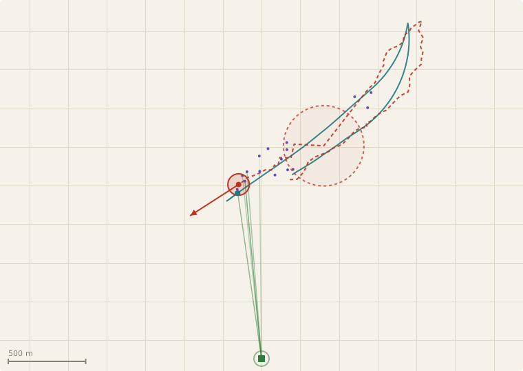
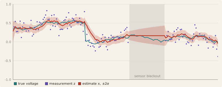
With JavaScript on, these become one live playground: a ship you steer through fog with the arrow keys, and the 1-D strip chart you can drag, both with sliders for R and Q and a live readout of the Kalman gain.

The assumption

Everything above is exact, genuinely optimal, not an approximation, for a linear system with Gaussian noise. Nothing in this post is a heuristic.

The catch is the sentence on page 2. The belief is carried as a mean and a variance, which is a complete description of a Gaussian and of nothing else. That is fine while $f$ and $h$ are linear, because a Gaussian pushed through a linear map is still a Gaussian. The moment they are not, the filter linearises them, keeps propagating a mean and a variance, and quietly asserts that the posterior is still bell-shaped.

Sometimes that is true enough. Sometimes the posterior has two peaks, the filter reports a single mean sitting in the valley between them, and it is not.

That gap is what the next three posts in this series are about: the extended Kalman filter and the lie it tells, the particle filter that carries the whole distribution as a cloud of samples instead of two numbers, and the experiment where the report plots the EKF’s Gaussian on top of the particle histogram and you can watch it miss the mode entirely.

But the scalar filter above is the part I would still write out from memory. Predict, inflate, weigh the innovation by an optimal step size, shrink. Everything after it is bookkeeping about how to keep doing that when the world is not linear.