Blog · Bayesian filtering ·
The Extended Kalman Filter, and the lie it tells
A first-order Taylor expansion, two Jacobians, and a filter that carries on as if the posterior were still Gaussian, shown on a lighthouse keeper tracking a ship from bearings alone, where it works beautifully and reports 46 m of cross-range confidence while sitting 680 m out along the beam.
- Interactive
- kalman-filter
- ekf
- state-estimation
- bayesian-filtering
- tracking
- python
The last post ended on the sentence the whole derivation rests on: the belief about the state is carried as a mean and a covariance, which is a complete description of a Gaussian and of nothing else. That is exact, genuinely optimal and not an approximation, as long as and are linear, because a Gaussian pushed through a linear map comes out a Gaussian.
The moment either of them bends, the algebra stops working. There is no closed form for the mean of of a Gaussian, never mind its covariance, and the posterior after one nonlinear measurement is generally not bell-shaped at all.
The Extended Kalman Filter’s answer to this is not subtle. It takes a first-order Taylor expansion of and about the current estimate, substitutes the derivative matrices wherever the linear filter used and , and carries on. Everything downstream (the gain, the covariance update, the claim that the result is a mean and a covariance of a Gaussian posterior) is then a statement about the linearised system, not about the real one. It is the same two lines of arithmetic, told a small lie about the world.
Sometimes the lie costs nothing. On the report’s dataset A the EKF is the best of all eight algorithms tested, particle filters included. On the bearings-only problem two posts from now it is about a thousand times worse than the plainest particle filter in the same table. This post is about why the first happens, and the widget below is about how the second one starts.
Where the Jacobians come from
The model is unchanged from post 17, Eqs (2.1) and (2.2), now with and allowed to be anything differentiable:
with and zero-mean and covariances and . §2 of the report expands both functions to first order, about the last posterior mean and about the prediction , Eqs (2.3) and (2.4):
and are Eqs (2.5) and (2.6), and they are nothing more exotic than the tables of partial derivatives you would write down by hand:
is square, . is : one row per number the sensor reports, one column per number you are estimating. It is usually very wide and very short, and that shape is the whole story of the second half of this post.
The two useful consequences follow in three lines each. The expected value of the propagated state, Eq. (2.7), is just of the mean, because the expected error is zero by construction:
and the prediction error, Eq. (2.8), propagates through the linearisation rather than through : , which squares up to Eq. (2.9):
That is the substitution, and it is the whole trick. From here the correction is identical to the linear case with in place of : the mean is nudged by the innovation, Eq. (2.10),
and the gain that minimises the trace of the posterior covariance, Eqs (2.12) and (2.13), is
Look at what survived and what did not. The mean goes through the real and the real : line 2 of Algorithm 1 and line 3 of Algorithm 2 below both call the honest function. The covariance only ever sees the Jacobians. So the estimate follows the curve and the uncertainty is computed on a tangent line, and nothing in the algorithm ever compares the two.
The algorithms, as the report boxes them
§2.1, printed page 4, transcribed:
Algorithm 1  EKF-Prediction(x[k-1], P[k-1])
  1   xf[k] <- f(x[k-1])
  2   Pf[k] <- Jf · P[k-1] · Jfᵀ + Q[k-1]
  3   return xf[k], Pf[k]

Algorithm 2  EKF-Correction(xf[k], Pf[k], z[k])
  1   K[k]  <- Pf[k] · Jhᵀ · (Jh · Pf[k] · Jhᵀ + R[k])⁻¹
  2   x[k]  <- xf[k] + K[k] · (z[k] − h(xf[k]))
  3   P[k]  <- (I − K[k] · Jh) · Pf[k]
  4   return x[k], P[k]
Side by side with post 17’s boxes they are the same seven lines; only the arguments of
, and the Jacobians moved. And ExtendedKalmanFilter.py is the same seven lines
again: this is predict (lines 39–42) and correction (lines 54–60) with the
docstrings removed:
def predict(self, xk_1pa, Pk_1, k=0):
    x_kpf = self.f(xk_1pa, k)
    Jf = self.Jf(xk_1pa, k)
    P_kpf = np.dot(Jf, np.dot(Pk_1, Jf.T)) + self.Q
    return x_kpf, P_kpf

def correction(self, x_kpf, P_kpf, zk, k=0):
    Jh = self.Jh(x_kpf, k)
    PJHT = np.dot(P_kpf, Jh.T)
    invM = np.linalg.inv(np.dot(Jh, PJHT) + self.R)
    Kk = np.dot(PJHT, invM)
    xkpa = x_kpf + np.dot(Kk, zk - self.h(x_kpf, k))
    Pk = np.dot(self.I - np.dot(Kk, Jh), P_kpf)
    return xkpa, Pk, Kk
Two details worth pointing at. Jf is evaluated at xk_1pa, the previous posterior,
before f moves the mean: that is what “expand about ” means, and
getting it the wrong way round is the classic EKF bug. And Jh is evaluated at
x_kpf, the prediction, because the correction has nothing better to linearise about yet.
A concrete : a lighthouse, and a ship
The report’s datasets are dimensionless and the post 17 example was a radar giving positions, which keeps everything linear. The smallest honest nonlinear sensor I can think of is a lighthouse keeper with a compass and no rangefinder.
The keeper sees one number per sighting: the bearing to the ship. The state is still four numbers, position and velocity, because velocity is what carries the estimate between sightings:
with the lighthouse. Write , and , differentiate, and is a single row:
Spend a moment on that row, because everything the widget does is written in it.
- The two trailing zeros say a bearing carries no direct information about velocity. Whatever the filter learns about how fast the ship is going, it learns entirely through the off-diagonal terms of : the correlations built up by the constant-velocity model. There is no other route.
- The vector is the line of sight rotated by 90°. The gain therefore only ever moves the estimate across the line of sight. A bearing can tell you that you have the ship on the wrong side of the beam. It cannot tell you it is twice as far away as you think, because that direction is in the null space of and always will be.
- The says the same information is worth less the further out the ship is: an error of one degree is 17 m at a kilometre and 87 m at five.
That third point is a scale effect and it is fine; a filter can be told about it. The second one is not a scale effect. It is a statement that one whole direction of the state space is invisible to this sensor at this instant, and the only thing that ever fills it in is the ship changing what it is doing.
Play with it
Two scenarios over the same filter. The lighthouse is the one above; dataset A is the report’s §4.1 problem replayed step for step, with its Table 1 numbers next to a live run so you can see what a single run of the thing behind those numbers looks like.
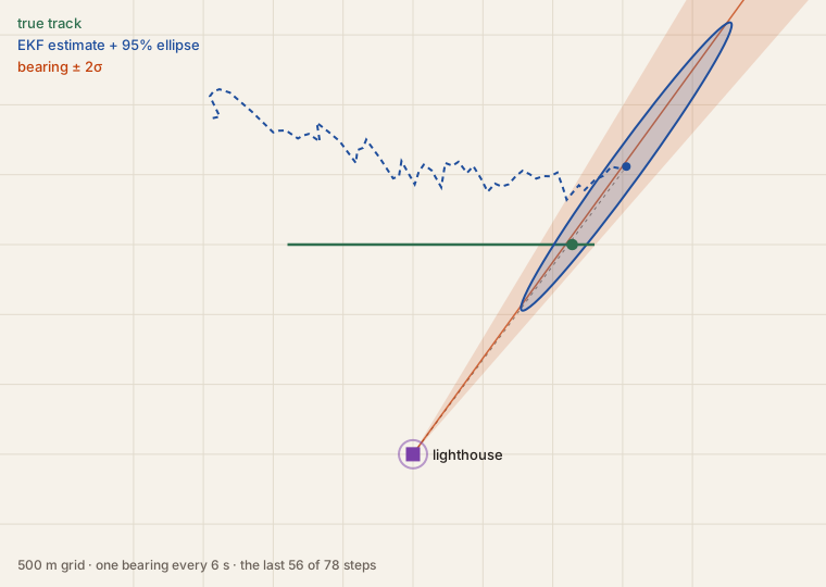
With JavaScript on, this becomes a ship you can steer past a lighthouse that can only see its bearing, with the EKF’s estimate and 95% ellipse updating every step, plus a replay of the report’s own dataset A.
On the lighthouse. Drag the chart to steer, or click it and use the arrow keys. The filter never sees the helm; every turn arrives at it as unmodelled acceleration.
-
Watch the ellipse. It is a cigar, and it points at the lighthouse. That is ‘s null space drawn to scale: the bearing pins the estimate across the beam and leaves it free along it. In the picture above the filter’s own numbers are σ = 46 m across the line of sight and σ = 520 m along it, an 11:1 ratio, and it is 680 m wrong, along the beam, of course.
-
Leave the ferry alone and nothing gets better, until the wall. Press Play and read the range error. On the default seed it goes 394 m at step 10, 880 at 30, 600 at 60, 1112 at 100, with σ along the beam growing the whole way. It is not converging slowly; it is not converging. With a stationary observer and a target that really is going in a straight line, scaling the entire trajectory about the lighthouse by any factor produces exactly the same bearings at exactly the same times: close-and-slow and far-and-fast are the same measurement history. Range is unobservable, and no quantity of data fixes an unobservable state.
Then at step 99 the ferry reaches the end of the channel and comes about, and that one turn does what the previous hundred sightings could not: by step 110 the range error is 8 m and σ along the beam has fallen from 733 m to 364. Manoeuvre, or stay ignorant is the entire operational doctrine of bearings-only tracking, and the ferry demonstrates both halves of it without being touched.
-
The trawler never stops turning, so it is never unobservable: over two hundred steps it settles at σ = 259 m along the beam against the ferry’s 601. The yacht’s tacks are gentler, and on the default seed it ends up worse than either at 731 m, a fair warning that “manoeuvre” here means a real alteration of course and not a wiggle.
-
Watch the innovation chart while you do all of this. It stays inside its ±2σ band the whole time the estimate is 680 m out. Over two hundred steps, 97% of the ferry’s innovations and 94% of the yacht’s fall inside it, which is about what a correctly calibrated filter should report. It has to: the estimate is on the right bearing, and the bearing is all the sensor measures. A filter cannot detect an error in a direction it cannot see, and a healthy innovation is not evidence that the answer is right, only that it is consistent with the measurements, which is a much weaker claim and one that is trivially satisfied here.
-
Switch the correction step to the IEKF and the innovation readout goes to exactly
0.00°and stays there, at a dozen or two passes a step. That is not the filter getting better; it is the loop in the next section reproducing each noisy reading perfectly. Keep it in mind while reading what follows. -
Hold Fog. The corrections stop, the estimate coasts on the velocity it last believed in, and the ellipse grows in both directions, because is isotropic and there is no bearing to squash it with. Let go and the next sighting flattens it back into a cigar in one step.
The IEKF, and what it actually does
There is an obvious improvement available. The correction linearises about , the prediction, but once the correction has run you have a better point to linearise about, namely the answer. So do it again. Keep doing it until the answer stops moving. That is the Iterated EKF, Algorithm 3, printed page 4:
Algorithm 3  IEKF-Correction(xf[k], Pf[k], z[k], α)
  1   x[k] <- xf[k]
  2   repeat
  3       xh[k]        <- x[k]
  4       x[k], P[k]   <- EKF-Correction(x[k], Pf[k], z[k])
  5   until ‖xh[k] − x[k]‖ < α
  6   return x[k], P[k]
and IteratedExtendedKalmanFilter.correction, lines 80–88, is that verbatim:
def correction(self, x_kpf, P_kpf, zk, k=0):
    prevx = x_kpf
    xkpa, Pk, Kk = ExtendedKalmanFilter.correction(self, x_kpf, P_kpf, zk, k)
    diff = prevx - xkpa
    while (diff * diff).sum() > self.thresh:
        prevx = xkpa.copy()
        xkpa, Pk, Kk = ExtendedKalmanFilter.correction(self, xkpa, P_kpf, zk, k)
        diff = prevx - xkpa
    return xkpa, Pk, Kk
self.thresh defaults to 1e-6, and note that the test is on
(diff * diff).sum(), the squared norm, so the real tolerance on is
, not .
It should help. On dataset A it does the opposite:
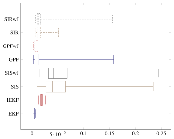
Figure 1, page 14: the same 100 runs behind Table 1, drawn as boxes. The EKF’s spread is a sliver; the particle filters’ whiskers run out to 0.25. The x axis is unlabelled in the original and is the per-run error in absolute units.
The report’s explanation, §7, page 24, is one sentence: “the multiple calls to the correction step of the algorithm can cause the algorithm to diverge. Hence, accuracy is gained at the cost of stability.” That is true and it is the right instinct. But porting the thing gave me a sharper answer, and it is worth writing down because it changes what the number means.
Look at what Algorithm 3 iterates. Line 4 calls EKF-Correction(x[k], Pf[k], z[k]),
the current answer as the first argument, where the prior mean used
to be. So the second pass computes
and the prior mean has vanished from the update entirely. The fixed point of that iteration is wherever , and has full column rank, so the fixed point is exactly. The loop does not refine the estimate towards a better linearisation of the posterior. It runs Newton’s method on the measurement equation until the filter reproduces this step’s noisy reading perfectly, and then stops. The prior gets applied once, on the first pass, and is then iterated away.
The textbook IEKF (Bell & Cathey, 1993) does not do this. It re-anchors on the prior mean every pass, with the extra term that keeps the prior in the picture:
The widget runs all three: the lighthouse has it as a third radio button, and dataset A draws it on request with Show re-anchored IEKF. Three things fall out of a hundred-run replay of Experiment 1 through my port, and all three are checkable in the widget:
- The EKF comes out at against the report’s 4.33, and the IEKF at against the report’s 18.06. Different random draws, same filters.
- Estimating and by simply inverting the measurement, solving and throwing the prior away, scores over the same hundred runs. The IEKF’s 18.06 is essentially that number, not a filtering result. It is measuring how badly the mixing matrix amplifies the measurement noise: with , , and nothing there has anything to do with sequential estimation. The small gap to 18.06 is the last bit of prior the stopping tolerance leaves behind.
- The re-anchored version scores , identical to the EKF, to the last digit, in two passes. It has to be: dataset A’s is exactly linear, so there is nothing to re-linearise and a correct IEKF must return the EKF’s answer.
So on this dataset “accuracy is gained at the cost of stability” is not quite the right diagnosis of the 18.06. Nothing diverged; the loop converged, quickly and reliably, to the wrong estimator. The report’s sentence is exactly right about the general risk (iterating a correction can and does diverge), but the 4.2× here is a missing term, not an instability. I am fairly confident of this reading; it is a 2026 note on 2018 code, and what I can prove is the arithmetic in the three points above, which you can re-run in the widget.
Dataset A, and why the EKF wins there
The problem the report’s headline number comes from, §4.1, printed page 7: , , , and with and :
with , and the filters all started at the origin knowing nothing. Two phases ramp linearly, and ; two sinusoids ride on them; a fixed 2×4 matrix mixes the sinusoids into a two-number measurement, and the filter has to unmix them.
Why is this easy? Because is a constant matrix. Its Jacobian does not depend on the state at all, the first-order expansion of it is not an approximation but an identity, and the correction step is exactly the linear Kalman filter’s. The only nonlinearity in the whole problem is in , where the sines and cosines live, and ‘s job is only to propagate the mean, which it does honestly. §7 puts it plainly: “This is due to the simplicity of the measurement function, h(x), as the EKF’s first order approximation is accurate. Furthermore, this example only has one possible mode of answers.”
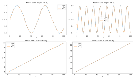
Figure 2, page 15: one run of the EKF on dataset A. The estimate is on top of the truth everywhere except the first two or three steps, where it is recovering from being started at the origin. This is what a Gaussian posterior looks like when it really is one.
Run the same thing in the widget’s second scenario and you get this figure back, live, with the IEKF drawn over it and the running error next to Table 1’s column. The metric is worth naming precisely, because the report does not:
What this buys, and what it does not
The EKF is not a bad algorithm. On a problem with a mild nonlinearity and a single mode it is the best thing in the report, better than eight thousand particles, and it costs one small matrix inverse a step. When it is right, it is right cheaply.
What it cannot do is tell you when it is not. The covariance it reports is computed from , , and alone, never from how wrong the answer actually turned out to be, so a filter that has committed to the wrong range reports a small, confident, beautifully-shaped ellipse around it, and an innovation sitting neatly inside its ±2σ band. Everything looks healthy. The Gaussian is a shape that has exactly one peak, and if the truth is that there are two places the ship could be, the filter’s only available answer is a single mean somewhere between them, with a covariance that describes neither.
That is the next post: what the posterior of a bearings-only problem actually looks like, why it has two peaks, and what four thousand weighted samples can represent that a mean and a covariance cannot.