Blog · Handwritten digits ·
Naive Bayes: the dumbest classifier that works
Assume sixty-four features are mutually independent, which they flatly are not, multiply their likelihoods and take the argmax. It reads handwriting at 89.97%, and two lines of the implementation are doing most of the work.
- Interactive
- naive-bayes
- mnist
- probability
- classification
- wasm
The previous two posts were about looking at a digit: tracing its contours and measuring them, then counting its gradients. This one is about deciding what the digit is, and the algorithm that does it is almost insultingly simple. Take the sixty-four numbers those two posts produce. Assume, falsely, obviously, self-evidently falsely, that every one of them is independent of every other. Multiply their likelihoods together. Take the biggest.
It reads MNIST at 89.97%.
A month and a bit later I would spend two assignments building a neural network from scratch, implement nine optimisers to train it, pick the best one, point it at the same dataset and score 70.19%. That comparison is the subject of a later post. This one is about why the dumb thing works.
Bayes’ rule, and then the lie
We want : the probability that a digit whose measurements are belongs to class . Bayes gives it to us directly:
The denominator does not depend on , so it cannot change which class wins; it only rescales. And MNIST’s ten classes are close enough to equally common that the prior is near flat. Both drop out, and what is left is a proportionality:
Extend that to all features at once and you get the thing we actually want to compute:
which is where the trouble starts, because is a joint distribution over a 64-dimensional space and there is no honest way to estimate it from 60,000 examples. So we lie:
Every feature is assumed independent of every other, given the class. This is not true. The arc length of a digit’s outline and the long side of its bounding box are obviously correlated; so are two HOG bins in neighbouring cells. The report I wrote at the time put it politely: “this requires that features should not depend on similar data, which is not always practically possible.” Then it said the useful thing, which is that the assumption is survivable. Modelling the real joint distribution costs exponentially more computation and exponentially more data, and buys you, in practice, a few percent. It is a trade, and the naive side of the trade is a product of one-dimensional histograms you can fit in an afternoon.
The naivety also has a nice side effect worth noticing: because each factor is estimated independently, adding a sixty-fifth feature costs one more histogram and one more multiplication. Nothing has to be refitted.
Two ways to estimate p(x|c)
Given the product, all that remains is a way to get out of the training set for one feature at a time. There are two cases, and they need genuinely different machinery.
Discrete: count, and divide
If takes one of values, , then the estimate is just a ratio of counts:
where is how many training digits had value and class , and is how many had class . That is a matrix and a counter. Training is one pass:
initialise: an (K+1) x 10 matrix, every cell set to 1
observe(x, c):
    j <- the row x falls in
    i <- the column for class c
    table[j][i] <- table[j][i] + 1
predict(x):
    row <- table[bin(x)]
    return row / sum(row)
Continuous features get binned first so they can use the same machinery: arc length is a real number, and the model turns it into “which of 196 half-unit-wide buckets does it land in”.
Continuous: fit a Gaussian per class
For the features that were left continuous (the eight image moments and the forty-eight HOG dimensions), the report assumes a shape for the density instead of binning it:
with the parameters estimated per class from the training data:
Ten Gaussians per feature, one per class, and the likelihood of a new measurement is where it falls under each. Normalising those ten values so they sum to one recovers . This is a real assumption and it is sometimes wrong (several of these features are visibly bimodal), but it costs two numbers per class instead of six hundred, and it works.
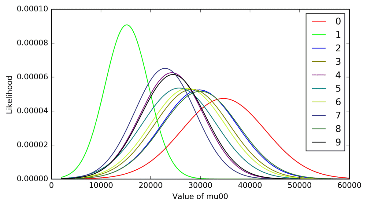
The report’s own plot of the ten fitted Gaussians for one feature: the m00 moment of the
deskewed digit. Each curve is one class’s . Where they
separate, the feature is informative; where they pile on top of each other, it is not. This
one is doing real work at the tails and almost nothing in the middle.
(Figs/P2/Momentmu00.png.)
The two lines that actually matter
Everything above is textbook. Two implementation details are not, and both of them are one line long.
One: initialise the counts to 1
PartBFeatureTypes.py:7-19, and the whole argument is the last line:
class classedFeature:
    def __init__(self, inputLabels, binned=False, outputLabels=list(range(10)), priorInit=True):

        self.inputLabels=inputLabels
        self.outputLabels=outputLabels
        self.binned=binned

        inCount=len(self.inputLabels) + 1 if binned else len(self.inputLabels)
        outCount=len(self.outputLabels)

self.countTable= np.ones((inCount,outCount)) if priorInit else np.zeros((inCount,outCount))np.ones, not np.zeros. Consider what happens without it. The areaEnclosed feature has 601
rows and there are ten classes, so its table has 6,010 cells; 60,000 training digits cannot
possibly populate all of them. Some (bin, class) pair will never be seen. Its count is zero, so
its estimated probability is zero, so when the reader draws a digit that lands in that bin, the
product
is zero for that class, no matter how confidently the other sixty-three features vote for it. One unlucky bucket in one feature vetoes the entire ensemble. Starting every cell at 1 (Laplace smoothing, though the report does not call it that) turns “impossible” into “as unlikely as a single observation”, which is what it actually is. It costs 9,390 additions at startup.
The + 1 in inCount on the line above matters for the same reason, incidentally: a binned
feature gets one extra row for everything past the last edge, so a value off the end of the
scale still has somewhere to land.
Two: divide by N − 1
PartBFeatureTypes.py:146-150, the whole of getTrainedFeature:
    def getTrainedFeature(self):
        vmean=np.vectorize(np.mean)
        vstd=np.vectorize(lambda x: np.std(x,ddof=1))

return trainedContinousFeature(vmean(self.storedValues), vstd(self.storedValues), self.outputLabels)ddof=1. NumPy’s default is ddof=0, which divides by and gives you the population
standard deviation of the sample you happen to have. That is biased low, because the sample
mean is by construction the point that minimises the squared deviations of that sample: one
degree of freedom has already been spent fitting it. Divide by and the estimate is
unbiased.
At per class the difference is one part in twelve thousand and could not possibly change a prediction. It is still the right line to write, and the report calls it out explicitly, which is the part I am still pleased about eight years later: “it is important to notice the minus 1 in the denominator, as this accounts for the degree of freedom used when fitting the mean to the data.”
Where the bins came from
TrainOnMetadata.py:12-33 is the entire configuration of the model, one line per feature,
each a hand-chosen range and step:
    pixelCount=classedFeature(np.arange(20,270,1).tolist(),True)
    arkLen=classedFeature(np.arange(30,128,0.5).tolist(),True)
    #convexContours=classedFeature([True,False])
    minLen=classedFeature(np.arange(4,28,0.5).tolist(),True)
    minWidth=classedFeature(np.arange(0,28,0.5).tolist(),True)
    minArea=classedFeature(np.arange(30,370,1).tolist(),True)
    ...
    numValidContours=classedFeature(np.arange(0,5,1).tolist(),True)
    areaEnclosed=classedFeature(np.arange(0,300,0.5).tolist(),True)
    VLines=classedFeature(np.arange(0,8,1).tolist(),True)
    HLines=classedFeature(np.arange(0,8,1).tolist(),True)
    cornerCount=classedFeature(np.arange(0,10,1).tolist(),True)
Every one of those ranges is a claim about the data. arkLen from 30 to 128 says no digit’s
outline is shorter than 30 pixels or longer than 128; cornerCount 0 to 10 says a digit has at
most ten Harris corners. The True is binned, which switches the lookup from an exact
list.index() to np.searchsorted:
    def getPclassesGivenFeature(self, featureValue):
        if self.binned:
            inputIndex=np.searchsorted(self.inputLabels,featureValue)
        else:
            inputIndex=self.inputLabels.index(featureValue)

        holdArr=self.countTable[inputIndex]

        return holdArr/np.sum(holdArr)
np.searchsorted with its default side='left' returns the number of edges strictly below the
value, which is exactly the bin index. For a value above every edge, it returns len(edges),
the overflow row the + 1 reserved. The two branches of that if are the whole difference
between a discrete feature and a binned continuous one.
Prediction: multiply, then argmax
PartBTest.py:40-70, trimmed of the commented-out lines but otherwise as written:
        posteriour=np.repeat(1/10,10)

        posteriour*=arkLen.getPclassesGivenFeature(imageDescriptor["arkLen"])
        posteriour*=minLen.getPclassesGivenFeature(imageDescriptor["minLen"])
        posteriour*=minWidth.getPclassesGivenFeature(imageDescriptor["minWidth"])
        posteriour*=numValidContours.getPclassesGivenFeature(imageDescriptor["numValidContours"])
        posteriour*=areaEnclosed.getPclassesGivenFeature(imageDescriptor["areaEnclosed"])
        posteriour*=VLines.getPclassesGivenFeature(imageDescriptor["VLines"])
        posteriour*=HLines.getPclassesGivenFeature(imageDescriptor["HLines"])
        posteriour*=cornerCount.getPclassesGivenFeature(imageDescriptor["cornerCount"])

        for i,hog in enumerate(Hogfeatures):
            posteriour*=hog.getPclassesGivenFeature(imageDescriptor["HOG"+str(i)])
        for k,f in zip(momentFeatureKeys,momentFeatures):
            posteriour*=f.getPclassesGivenFeature(imageDescriptor[k])

        posteriour/=np.sum(posteriour)
        predicted=np.argmax(posteriour)
That is the classifier. A flat prior, sixty-four multiplications, one normalisation, one argmax.
Three things in that block are worth pointing at.
Not every feature that gets computed gets used. GenerateDescriptors.py extracts
pixelCount, minArea and seven Hu moments for every one of the 70,000 digits, and at
inference all ten of those lines are commented out (PartBTest.py:42-43, 50-51, 62-63).
TrainOnMetadata.py still trains pixelCount and minArea and still writes them into the
model file; only huM0 of the seven Hu moments is even serialised, and it is commented out too.
So the shipped model carries two features nothing reads, and the extraction pass spends its time
computing seven rotation-invariant moments that never reach a decision. Dead weight, but honest
dead weight: the code says so, in place, rather than pretending.
The /= np.sum() is at the bottom, not in the loop. Interleaved between every line of that
block, in the committed source, is a commented-out posteriour/=np.sum(posteriour). Somebody
(me) clearly hit a numerical problem, tried renormalising after every factor, and then commented
it all out again. The instinct was right and the fix was clumsy. Sixty-four factors each around
0.1 gives a product around , which float64 holds comfortably; but a digit that is
genuinely unlike its class can push individual factors to , and then a few dozen of
them multiplied together is -ish and you are one bad feature away from a row of
exact zeros and an argmax that silently returns 0.
In the port, that is not a judgement call. Sum logarithms instead of multiplying probabilities and the problem does not exist:
Exponentiate once, at the end, after subtracting the maximum. bayes.rs does this, and a test
asserts both halves: that the log-domain answer matches a direct float64 product on a case small
enough not to underflow, and that it still returns a confident 7 on a case where the direct
product underflows to exactly zero for all ten classes.
Draw one
Everything above, running in your browser. Draw a digit, or load a real MNIST test digit if you would rather see what the model was trained on, and the ten bars are the posterior, live.
The panel underneath is the part I would actually keep. Each row is one group of features showing its own ten-way verdict, computed from that group alone, and each has a checkbox. Untick HOG and watch the accuracy readout fall off a cliff. Untick contour count and 8s start reading as 3s, because the thing that tells an 8 from a 3 is that an 8 has two holes in it and that is the only feature measuring holes. Untick everything and you get a flat 10%, the prior, which is the honest answer when you have looked at nothing.
With JavaScript on, this is a canvas you can draw a digit on. Ten bars show the classifier’s posterior probability for each class as you draw, and eight checkboxes let you switch feature groups (arc length, min-area box, contour count, enclosed area, Hough lines, corner count, image moments and the 48 HOG dimensions) in and out of the product, with the held-out accuracy recomputed from 1,000 MNIST test digits each time.
The two thumbnails under the canvas are the preprocessing, and they matter more than they look. The first is your drawing put into the form MNIST actually distributes: cropped to its bounding box, scaled so the longer side is 20 pixels, and translated so its centre of mass sits at the centre of a 28×28 field. Demos that skip that step and just squash the canvas to 28×28 hand the model digits that are the wrong size and off-centre, and then wonder why nothing works. The second thumbnail is the 32×32 perspective deskew from the feature-engineering post: every moment and every HOG bin is measured on that, not on your drawing.
What it got right, and what it got wrong
The report’s confusion matrix, transcribed. Rows are the true label, columns the predicted one; 89.97% is the trace over the total.
| true \ pred | 0 | 1 | 2 | 3 | 4 | 5 | 6 | 7 | 8 | 9 |
|---|---|---|---|---|---|---|---|---|---|---|
| 0 | 915 | 2 | 13 | 8 | 0 | 4 | 15 | 0 | 20 | 3 |
| 1 | 0 | 1075 | 19 | 2 | 13 | 1 | 0 | 5 | 19 | 1 |
| 2 | 9 | 1 | 956 | 29 | 3 | 2 | 0 | 4 | 27 | 1 |
| 3 | 0 | 2 | 26 | 925 | 2 | 23 | 1 | 7 | 16 | 8 |
| 4 | 0 | 7 | 27 | 0 | 892 | 2 | 10 | 8 | 5 | 31 |
| 5 | 7 | 0 | 7 | 50 | 3 | 777 | 10 | 2 | 32 | 4 |
| 6 | 10 | 10 | 7 | 1 | 9 | 26 | 881 | 0 | 14 | 0 |
| 7 | 0 | 6 | 35 | 10 | 32 | 0 | 0 | 842 | 10 | 93 |
| 8 | 30 | 9 | 23 | 26 | 9 | 16 | 2 | 11 | 828 | 20 |
| 9 | 9 | 9 | 17 | 10 | 8 | 8 | 0 | 26 | 16 | 906 |
The dominant failure is 7 against 9: 93 sevens called nines and 26 nines called sevens, 119 images, 1.19% of the whole test set in one confusion. The report predicted that before running the experiment: “one could expect to see many misclassification of the digit ‘7’ and ‘9’ as these two digits are very similar in structure,” which is the cheapest kind of correct prediction to make, but it was written down first. After that: 50 fives called threes, 35 sevens called twos, 32 sevens called fours, 32 fives called eights, 31 fours called nines, 30 eights called zeros.
The other thing the matrix says is that class 5 is the weakest: 777 of 892 fives found, an 87% recall against 95% for 1s. A five has no enclosed area, an ambiguous corner count and an arc length that overlaps almost everything: of the eight feature groups, nothing in the list is about a five.
How reliable is 89.97%?
This is the part of the report I like best, because it is the question almost nobody asks about their own accuracy number. 89.97% is one measurement on one test set. What would it have been on a different ten thousand digits?
The experiment: score all 10,000 test digits once, keeping a 1 or a 0 per digit. Then draw 1,000 of those flags at random without replacement, average them, and write down the result. Repeat 100,000 times. The spread of that distribution is an estimate of how much the headline number depends on which digits you happened to be handed.
The answer, from the report’s box plot:
| median | lower quartile | upper quartile | lower whisker | upper whisker | |
|---|---|---|---|---|---|
| accuracy | 90.0% | 89.4% | 90.6% | 85.3% | 93.9% |
| certainty | 89.93% | 89.33% | 90.53% | 85.97% | 93.57% |
Half of all resamples land between 89.4% and 90.6%, so the second decimal place of “89.97%” is noise and the first is not. And the worst thousand digits you could be handed still score above 85%, which is the useful form of the claim: this will probably be at least 85% correct on your data too.
The second row is a different measurement and it is the one worth a paragraph. “Certainty” here is the probability the classifier assigned to the correct label, averaged the same way: not whether it was right, but how much of its belief it put on the truth. Its median is 89.93% against an accuracy median of 90.0%. The two distributions sit on top of each other.
That means the classifier is neither over- nor under-confident. When it says 90%, it is right about 90% of the time. A model that scored 90% while claiming 99% would be dangerous in a way this one is not, and for something built out of sixty-four histograms under an assumption that is flatly false, being that well calibrated is a genuinely nice property. It is also a little lucky: nothing in the training procedure was trying to achieve it.
Run it yourself, on my model’s outcomes rather than the 2018 ones:
With JavaScript on, this resamples 1,000 of the 10,000 stored test outcomes without replacement, tens of thousands of times, and draws the resulting box plot for both accuracy and certainty, against the five numbers the 2018 report published.
Push “digits per sample” down to 100 and the box gets dramatically wider: a hundred-digit test set tells you almost nothing about the second digit of your accuracy. That is the whole lesson of the experiment in one slider.
What I could and could not reproduce
Three separate problems, in the order I hit them.
The trained model was never committed. TrainOnMetadata.py writes trained/Trained.dat;
the trained/ directory is not in the repository, and neither is the intermediate
meta/Intermidiate.dat the training reads. This turns out not to matter, because all four MNIST
idx files are committed (53 MB of them), so the whole pipeline can be re-run from the top.
The committed code disagrees with itself about how many HOG dimensions there are.
TrainOnMetadata.py:32-33 reads
    Hogfeatures=[]
    #for i in range(48):
    for i in range(9):
and PartBTest.py:22 reads for i in range(48):. Run the two as committed and the test crashes
on a missing HOG9 key. They cannot both be right, so before quoting any accuracy I had to work
out which one produced 89.97%. The evidence:
- The
cv2.HOGDescriptorinGenerateDescriptors.py:14-28is configuredwinSize=(32,32),blockSize=(16,16),blockStride=(16,16),cellSize=(16,16),nbins=6. That is 2×2 = 4 block positions, one cell each, six bins: 24 dimensions. Neither 9 nor 48. - Directly above those two lines sit their commented-out alternatives:
#cellSize = (8,8)and#nbins = 3. With both uncommented the arithmetic is 4 blocks × 4 cells × 3 bins = 48. No other combination of the values present in that file produces 48. Figs/P2/HOG24.pngexists. The plotting loop that produced it iterates over every trained HOG feature, so at the time the figures were made there were at least 25 of them.
So: the run that produced 89.97% used a 48-dimensional HOG from 8×8 cells with 3 orientation
bins, PartBTest.py:22 is the line consistent with it, and the range(9) in TrainOnMetadata
is a later edit, almost certainly made to stop the script opening forty-eight matplotlib
windows in a row, since the line right after it plots every feature it trained. I have used
48 dimensions at 8×8 cells and 3 bins throughout.
The extractor is mine, not OpenCV’s. A naive Bayes model is nothing but a summary of the
features it was trained on, so shipping a model trained on OpenCV’s numbers and then measuring
digits with a hand-rolled reimplementation in the browser would produce a demo that quietly
misclassified everything. The only correct move is to train with the same code the browser
runs, which is what I did: the model on this page was trained by digits-wasm’s own
bayes.rs::extract, calling the contour tracer, min-area rect and perspective warp from
post 3 and the descriptor from
post 4, over all 60,000 training digits.
The differences from OpenCV are real and are documented next to each kernel: the Moore-neighbour
tracer finds holes by flood fill rather than by RETR_TREE’s contour hierarchy, the HOG skips
OpenCV’s Gaussian block weighting and spatial trilinear interpolation, the Harris threshold is a
fraction of the frame’s own peak rather than an absolute value on OpenCV’s internally-rescaled
response, and the “enclosed area” feature counts hole pixels directly instead of summing polygon
areas.
I assumed those differences were the whole of the 3.5-point gap. They are not, and finding that out is the most interesting thing in this post.
The published number does not reproduce
Having a working pipeline, the obvious check was to also re-run the original one. So I did:
GenerateDescriptors.py with OpenCV doing all the work, exactly as written except for the
OpenCV 3-to-4 change in what findContours returns, over all 70,000 digits; then
TrainOnMetadata.py’s tables and PartBTest.py’s product, transcribed into vectorised NumPy so
the whole sweep runs in seconds. Every bin edge, the np.ones initialisation and the ddof=1
are the originals’.
| pipeline | accuracy |
|---|---|
| the report, 2018 | 89.97% |
| OpenCV rerun, 48-dim HOG (8×8 cells, 3 bins) | 85.83% |
| OpenCV rerun, 24-dim HOG (16×16 cells, 6 bins) | 85.81% |
OpenCV rerun, 48-dim, plus pixelCount | 86.10% |
OpenCV rerun, 48-dim, plus pixelCount and minArea | 86.18% |
| OpenCV rerun, 48-dim, plus all seven Hu moments | 50.72% |
| this page’s Rust model | 86.43% |
Neither HOG configuration reaches the published figure, and neither does putting back any
combination of the features PartBTest.py leaves commented out: the best OpenCV run I can
produce is 86.18%, and switching the seven Hu moments back on is catastrophic, halving the
accuracy, which is presumably why they were commented out in the first place.
So the honest summary is not “my port loses 3.5 points to OpenCV”. It is that the committed code does not produce 89.97% today, by either route, and that my from-scratch extractor happens to land a fraction of a point above the OpenCV rerun rather than below it.
What I cannot tell you is why. trained/Trained.dat was never committed, so there is no model
to diff against; the repository has a single commit for all of the source, so there is no
history showing what GenerateDescriptors.py looked like on the day the report was written; and
the OpenCV I have is 4.10, not whatever 3.x was installed in 2018. Any of those could hold the
missing four points. I have quoted 89.97% throughout as what the report says, because that is
what it says, and 86.43% as what this page actually does, because that is what I measured.
What each feature is actually worth
Because the widget can re-score a held-out set with any subset of groups switched on, the ablation is free. On the 1,000 test digits shipped with this page, with my model:
| feature group | accuracy without it | accuracy from it alone |
|---|---|---|
| arc length | 87.5% | 35.5% |
| min-area box | 87.3% | 33.4% |
| contour count | 87.3% | 25.9% |
| enclosed area | 87.3% | 29.0% |
| Hough lines | 87.5% | 33.0% |
| corner count | 87.4% | 34.3% |
| image moments | 88.5% | 64.7% |
| HOG (48 dims) | 80.2% | 81.6% |
| all eight | – | 87.7% |
Two things jump out.
HOG carries the classifier. On its own it scores 81.6%, within six points of the whole ensemble; remove it and the other seven groups together manage 80.2%. The report saw the same thing in the information gain: HOG scores above 0.90 for every digit, where the hand-designed features each score 0.9 for one digit and near zero for the rest, and said outright that it “could even be used by itself”. It was right.
The image moments actively hurt. Removing them takes 87.7% to 88.5%. This is the
independence assumption presenting its bill: eight moments of the same 32×32 image are about as
far from mutually independent as features get (mu20, mu02 and m00 are three views of the
same blob), and multiplying eight correlated likelihoods counts the same evidence eight times
over. When that evidence is right it is merely redundant; when it is wrong it is eight votes
wrong. The six cheap geometric features each cost a few tenths of a point to remove, which is
what you would expect from features that measure genuinely different things.
I did not tune any of this. The feature list, the bin edges and the HOG configuration are the 2018 ones; the table is just what falls out.
The sequel loses
A month later I started the neural-network assignment: derive backpropagation from first principles, implement nine optimisers, benchmark them properly, take the best one, iRPROP+, and point a 784×100×10 network at MNIST. It scored 70.19%, nineteen points behind the histogram-multiplier I had written in March. The reason is not that neural networks are bad; it is a single hyperparameter in the stopping criterion, and finding it is the subject of that post.
The thing I took from having built both is smaller than either. The naive Bayes classifier has no free parameters at all. There is nothing to tune, no learning rate, no initialisation, no stopping criterion, and therefore nothing that can silently destroy the result while the code runs without error. It is the dumbest thing in the box, and being dumb is exactly why you can trust the number it gives you.