Blog · Classical ML ·
De-noising an image with a Markov random field, and 22 ways to shape its neighbourhood
Write down what you believe about images as an energy function and de-noising becomes minimising it. The interesting part is replacing the textbook four-neighbour smoothness term with an arbitrary kernel window, and then testing 22 of them.
- Interactive
- markov-random-fields
- graphical-models
- icm
- image-denoising
- wasm
Two things I believe about a scanned page: neighbouring pixels usually agree, ink is next to ink, paper is next to paper. And the scan I am holding is probably not far from the truth, however speckled it looks.
Neither belief is a filter. They are just opinions. But if you can write an opinion as a number that gets smaller when the opinion is satisfied, then adding up those numbers over a whole image gives you a single quantity to minimise, and de-noising stops being a recipe and becomes an optimisation problem. That number is called an energy, the machinery for writing it down is a Markov random field, and the cheapest way to minimise it is a rule that fits on one line.
This is Part C of the same assignment as the Gaussian process and SVM posts. Where it goes past the textbook is one substitution: Bishop’s smoothness term sums over a pixel’s four neighbours, and I replaced that with a weighted sum over an arbitrary kernel window. That one change turns “a smoothness prior” from a phrase into a shape you can draw, edit and compare, so I drew 22 of them and put the errors in a table.
The results are counterintuitive in a useful way. Bigger neighbourhoods are worse: a 3×3 all-ones window ends at 3.45% wrong pixels, a 17×17 one at 9.37%. Weighting neighbours by distance beats treating them equally at every single size. And a kernel that only looks up and down physically cannot remove noise that lies to its left and right, so it stalls after one sweep at 10.78% and never improves again.
Cliques, potentials, energies
A graphical model draws random variables as nodes and dependencies as links. Direct the links and you get a Bayesian network; leave them undirected and you get a Markov random field. The useful structure in an undirected graph is the clique: a set of nodes that are all connected to each other, and specifically the maximal cliques, the ones that are not contained in a bigger clique.
The joint distribution factorises over those maximal cliques:
with a normalising constant and a potential function on clique . A potential is not a probability; it just has to be positive. The standard way to guarantee that, and the reason any of this is tractable, is to write
Now the product of potentials is the exponential of a sum of energies, maximising the probability is minimising the total energy, and (which nobody can compute) drops out of every comparison you actually want to make.
The model: two grids, one link each
Take a binary image, pixels in . There is a hidden grid we want (the clean image), and an observed grid we have (the noisy one), made by flipping the sign of a fraction of the pixels at random. Two families of link: each is joined to its neighbours inside , and each is joined to its own . Both families are cliques of size two, so the energy is a sum of one term per link, and the only links a single pixel takes part in are the ones in the picture below.
Everything one ICM decision looks at. The estimate x is joined to its own observation y with weight η, and to the pixels in the kernel window with weight β times the kernel entry; h tilts the whole thing towards one colour. Setting the kernel to a plus shape recovers Bishop’s four-neighbour model.
The energy, and the one term I changed
The report’s Eq. (5.2), with meaning “sum over the image” and meaning “sum over the pixels adjacent to the current one”:
Three terms, three jobs.
- is a prior on colour. Positive makes the total smaller when more pixels are , so it biases the answer towards one of the two classes. Zero means a uniform prior.
- is agree with your neighbours. Two pixels of the same sign multiply to and so lower the energy; two that disagree raise it.
- is trust the observation, the same trick one link down.
And now the substitution. That inner sum over adjacent pixels is an unweighted sum over four neighbours. Replace it with a window function that takes the kernel-weighted sum of the neighbourhood against a matrix :
Setting to a plus shape recovers the textbook model exactly. Setting it to anything else is a different prior about what “smooth” means, and unlike the phrase, you can look straight at it.
Since and , and does not depend on , maximising the posterior is minimising .
Why the flip test is local
Iterated conditional modes is the laziest possible minimiser: walk over the pixels, and flip any one that lowers the energy. Naively that costs a full energy evaluation per pixel. It does not, because almost everything cancels. Writing and subtracting the two energies, every pixel except appears identically in both and drops out:
Flip when that is negative. It reads pixels and nothing else: no normalising constant, no global pass, no matrix. That is the entire algorithm.
Two algorithms, and why they disagree
The straightforward version sweeps the whole image until nothing changes:
Algorithm 1: ICM
 1  procedure ICM(I_y, K)
 2      I_x ← copy of I_y
 3      while not converged do
 4          for i, j in shape(I_x) do
 5              if ΔE(x_ij, y_ij, K) / 2 < 0 then
 6                  x_ij ← −x_ij
 7              end if
 8          end for
 9      end while
10      return I_x
11  end procedure
That reprocesses the whole image every round, and after the first sweep almost none of it can have changed. Only a pixel within the kernel footprint of something that just flipped can have a different answer this time, so keep a set of those instead:
Algorithm 2: ICM with a dirty set
 1  procedure ICM(I_y, K)
 2      I_x ← copy of I_y
 3      S ← {}
 4      for i, j in shape(I_x) do
 5          if ΔE(x_ij, y_ij, K) / 2 < 0 then
 6              x_ij ← −x_ij
 7              S ← S ∪ {indices in the vicinity of i, j}     ▷ a set: no duplicates
 8          end if
 9      end for
10      while S is not empty and no other termination condition is met do
11          i, j ← pop(S)
12          if ΔE(x_ij, y_ij, K) / 2 < 0 then
13              x_ij ← −x_ij
14              S ← S ∪ {indices in the vicinity of i, j}
15          end if
16      end while
17      return I_x
18  end procedure
The implementation keeps two sets, one for the current round and one being built for the next, purely so that “a sweep” stays a meaningful unit and each one can be drawn as a frame.
The code
The whole thing is about fifty lines of Python. This is GraphicalMethods/PcUtils.py
lines 22–27 and 39–44: the flip test with an arbitrary kernel, and the border handling it
leans on:
def calcHalfDeltaKernel(i,j,x,y,h,eta,B,kernel):

    return (-h*x[i,j]
            +B*x[i,j]*np.sum(np.multiply(kernel,
                getZeroPaddedKernel(int(len(kernel)/2.0),x,i,j)), axis=(0,1))
            +eta*x[i,j]*y[i,j])

def getZeroPaddedKernel(halfKernelSize,x,i,j):
    i1,i2=max(i-halfKernelSize,0),min(i+halfKernelSize+1,len(x))
    j1,j2=max(j-halfKernelSize,0),min(j+halfKernelSize+1,len(x[0]))
    outhold = np.zeros((2*halfKernelSize+1,2*halfKernelSize+1)+x.shape[2:])
    outhold[i1-i+halfKernelSize:i2-i+halfKernelSize,j1-j+halfKernelSize:j2-j+halfKernelSize]=x[i1:i2,j1:j2]
    return outhold
getZeroPaddedKernel is the whole border policy: outside the image counts as , so an edge
pixel simply sees fewer neighbours. It does not wrap and it does not mirror. (The three
hand-written specialisations above it in the same file, calcHalfDelta, calcHalfDelta2,
and calcHalfDelta3, index x[i-1,j] directly and therefore do wrap around the array on
the top and left edges. I never called them for any of the runs below, and I am glad, because
they are wrong.)
And the driver, Pc.py lines 194–211, which is Algorithm 2 spelled out with two Python sets:
for i in range(0,len(x)):
    for j in range(0,len(x[0])):
        if deltafn(i,j,x,y,h,eta,B) < 0:
            x[i,j]=-x[i,j]
            toCheck|=set(map(tuple,[i,j]+itemsToCheck))

while len(toCheck)>0:
    looper+=1
    showImage(x,looper,baseExperement)
    error=np.count_nonzero(x_gt-x)/x.size
    errors.append(error)
    toCheckNext=set()
    for i,j in toCheck:
        if -1 < i < len(y) and -1< j < len(y[0]):
            if deltafn(i,j,x,y,h,eta,B) < 0:
                x[i,j]=-x[i,j]
                toCheckNext|=set(map(tuple,[i,j]+itemsToCheck))
    toCheck=toCheckNext
For the widget I ported that to Rust, because I wanted it to run on a canvas you can draw on
rather than on one fixed 177×88 image, and a 400×300 canvas with a 17×17 window is
34.7 million multiply-adds per sweep. The port is the same
arithmetic over an i8 buffer:
/// `W(x, i, j)`: the kernel-weighted neighbourhood sum, zero-padded at the
/// border. Equivalent to `np.sum(kernel * getZeroPaddedKernel(...))`.
#[inline]
pub fn window(&self, i: usize, j: usize) -> f32 {
    let hk = self.ks / 2;
    let i0 = i.saturating_sub(hk);
    let i1 = (i + hk + 1).min(self.h);
    let j0 = j.saturating_sub(hk);
    let j1 = (j + hk + 1).min(self.w);
    let mut s = 0.0f32;
    for ii in i0..i1 {
        let krow = (ii + hk - i) * self.ks;
        let xrow = ii * self.w;
        for jj in j0..j1 {
            s += self.kernel[krow + jj + hk - j] * self.x[xrow + jj] as f32;
        }
    }
    s
}

/// `ΔE / 2` for flipping pixel (i, j), Eq. (5.3). Negative means flip.
#[inline]
pub fn half_delta(&self, i: usize, j: usize) -> f32 {
    let k = i * self.w + j;
    let xij = self.x[k] as f32;
    -self.prior_h * xij + self.beta * xij * self.window(i, j) + self.eta * xij * self.y[k] as f32
}
The dirty set became a Vec<u32> deduplicated by a stamped visited array, which is the only
place the port is not a transcription: a Python set of (i, j) tuples iterates in hash
order, and mine iterates in insertion order. That is exactly the order-of-operations
difference that moves the plus kernel by twelve hundredths of a percent.
The crate is 23.5 kB of WebAssembly and its test suite re-runs all 22 kernels against the report’s table; the largest disagreement across the whole of Table 8 is 0.09 percentage points.
The image
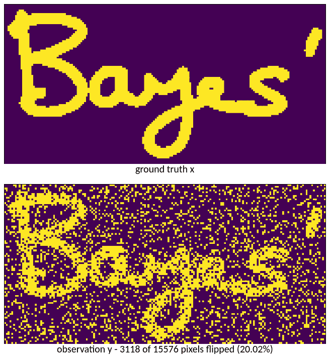
The assignment’s test image and its corrupted copy, straight out of the repo’s own
Outputs/OrigionalData/. 177×88 pixels; 3 118 of the 15 576 have had their sign flipped,
which is 20.02%.
Every parameter below was tuned by the particle swarm optimiser I had written for an earlier assignment, minimising the number of wrong pixels.
Drive it
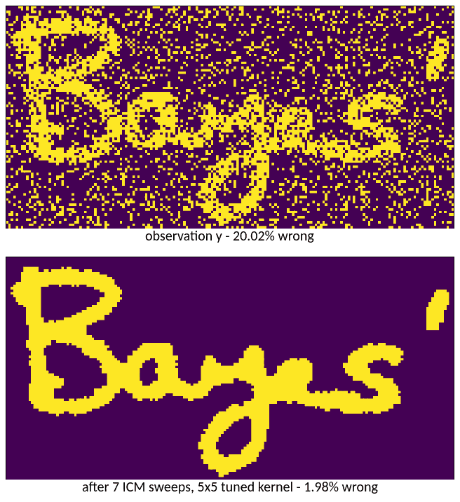
With JavaScript enabled this becomes a live bench: draw on the left canvas or upload your own scan, edit the kernel weights cell by cell, and step ICM one sweep at a time against a plot of the stored 2018 run.
Things worth doing to it:
- Press Step repeatedly. Flipped pixels flash, and you can watch the first sweep do almost all the work (20.02% to 4.17% for the plus kernel), and the following six argue about the edges.
- Press “η = 0”. The field stops listening to the observation and starts optimising the smoothness term alone. It does not converge to a blank image; it converges to blobs.
- Set the window to 17×17 all ones and watch the letters dissolve while the error climbs.
- Pick Vertical, run to convergence, and see it stop after a single sweep with horizontal streaks of noise it is structurally incapable of seeing.
- Upload a photo of your own handwriting. It gets thresholded to two colours and capped at 400×300; the tuned 5×5 kernel does a decent job on ink, and you can download the result.
The plot overlays your run against the errors.txt the 2018 experiment wrote for the same
kernel, so the dashed line is what the original run did and the solid line is what is
happening now. They are close but not identical, for the ordering reason above.
The kernel zoo
Table 7 of the report (p. 32), transcribed. · is a zero; the centre weight is always zero,
because a pixel is not its own neighbour.
| Kernel | Window | Free parameters |
|---|---|---|
| Vertical | · 1 · / · · · / · 1 · | none |
| Horizontal | · · · / 1 · 1 / · · · | none |
| Plus shaped | · 1 · / 1 · 1 / · 1 · | none |
| N×N all ones | every weight 1 | none |
| 3×3 adaptive | a 1 a / 1 · 1 / a 1 a | |
| Diamond | the 5×5 taxicab ball of radius 2 | none |
| 5×5 adaptive | p₁ p₂ p₃ p₂ p₁ / p₄ p₅ p₆ p₅ p₄ / p₇ p₈ · p₈ p₇ / … | , four-fold symmetric |
| N×N Gaussian | a bivariate normal sampled at each offset, then normalised to sum 1 | none |
The Gaussian’s weight at offset is with , the centre set to zero and the whole thing normalised. Note what that covariance does: it is , so a wider window is also a flatter one. The 17×17 Gaussian is not a tight blob inside a big window; it is genuinely spread across all 289 cells. That matters for the next section.
The results
Table 8 (p. 37), with a column for what the Rust port gets today, sorted best to worst. Both columns are the fraction of pixels that disagree with the ground truth after convergence, starting from 20.02%.
| Kernel | Report (%) | This port (%) |
|---|---|---|
| 5×5 adaptive | 1.98 | 1.98 |
| Diamond | 2.25 | 2.34 |
| 5×5 Gaussian | 2.28 | 2.24 |
| 7×7 Gaussian | 2.52 | 2.55 |
| 5×5 all ones | 2.56 | 2.49 |
| 3×3 adaptive | 2.84 | 2.88 |
| 3×3 Gaussian | 2.95 | 2.94 |
| Plus shaped | 3.15 | 3.20 |
| 9×9 Gaussian | 3.23 | 3.18 |
| 3×3 all ones | 3.45 | 3.43 |
| 11×11 Gaussian | 3.79 | 3.84 |
| 7×7 all ones | 4.08 | 4.07 |
| 13×13 Gaussian | 4.48 | 4.46 |
| 15×15 Gaussian | 5.12 | 5.06 |
| 17×17 Gaussian | 5.67 | 5.70 |
| 9×9 all ones | 5.80 | 5.80 |
| 11×11 all ones | 6.99 | 7.01 |
| 13×13 all ones | 8.28 | 8.29 |
| 15×15 all ones | 8.92 | 8.92 |
| 17×17 all ones | 9.37 | 9.37 |
| Horizontal | 10.62 | 10.62 |
| Vertical | 10.78 | 10.78 |
Three readings.
Distance-weighted beats uniform, at every size. Every Gaussian row beats the all-ones row of the same width, and it is not close: 2.24% against 2.49% at 5×5, 5.70% against 9.37% at 17×17. Telling a pixel that its far neighbours matter as much as its immediate ones is a bad prior about images.
Bigger is worse. Both families get monotonically worse from 5×5 upward. This is the opposite of the intuition you carry over from blurring, where a bigger kernel means more averaging and therefore less noise. Here a bigger window means a pixel’s value is decided by data further and further away, and an edge, which is exactly where the information is, gets pulled apart from both sides.
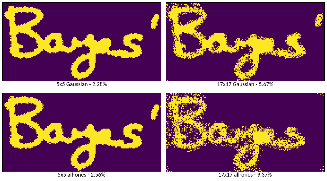
The same image, four windows. Left column 5×5, right column 17×17; top row Gaussian, bottom
row all-ones. Rendered by the original experiment into
GraphicalMethods/Outputs/.
A directional kernel is blind across its own axis. The vertical kernel sees only the
pixels above and below. A noisy pixel with a noisy pixel to its left is invisible to it, and
a vertical pair of flipped pixels is stable: each one supports the other. So it does one
sweep, fixes what it can see, and stops: 10.78%, from an errors.txt that has exactly two
entries in it. The horizontal kernel does the same thing rotated, at 10.62%.
A bug worth showing you
The all-ones kernel is built like this, in Pc.py lines 98–99:
kernel = np.ones((Ksize,Ksize))
kernel[2,2] = 0
That is meant to punch the centre out: a pixel should not be its own neighbour. It only
is the centre when Ksize is 5. At 3×3 it zeroes the bottom-right corner; at 17×17 it
zeroes a cell two rows and two columns in from the top left, and leaves the centre weight
at 1.
A non-zero centre weight puts into the flip test: a constant, because either way. It does not vanish; it biases every pixel against flipping at all, uniformly. And because the swarm tuned and against this shape, the tuned parameters absorbed it. Fixing the kernel without re-tuning makes things worse, not better:
| N | Table 8 | The kernel as written | Centre actually zeroed |
|---|---|---|---|
| 3 | 3.45 | 3.43 | 3.06 |
| 5 | 2.56 | 2.49 | 2.49 |
| 9 | 5.80 | 5.80 | 6.55 |
| 13 | 8.28 | 8.29 | 9.91 |
| 17 | 9.37 | 9.37 | 10.91 |
At 3×3 the correct kernel is genuinely better, and the repo contains a separate run of the
literal [[1,1,1],[1,0,1],[1,1,1]] with its own tuned , which lands at 3.06%, not
the 3.45% Table 8 reports. So one row of the published table is a number for a kernel that is
not the kernel the table describes. The widget ships both, and you can see the stray zero and
the live centre in the grid.
What each term actually does
Section 5.4 of the report answers this in prose. The repo answers it in three directories,
a1, a2 and a3, each one a run of the tuned 5×5 kernel with one term switched off. They
are all reproducible with one button in the widget.
η = 0, the field stops listening. With no data term, the only forces left are smoothness and the prior, and the noisy image is merely a starting point. Every pixel would rather agree with its neighbours than with anything, so agreement spreads. The error climbs from 20.02% to 30.43% over 52 sweeps, worse than doing nothing at all, and it ends in a picture that has nothing to do with the input.
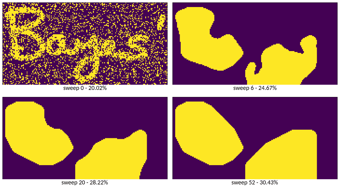
The a1 ablation: η = 0, so the estimate stops being anchored to the observation. Six
sweeps in, the word is gone and two blobs are negotiating a border. Forty-six sweeps later
they are still at it. The error over that run: 20.02% → 24.67% → 28.22% → 30.43%.
β = 0, nothing happens. With no smoothness term the flip test is
, and every pixel starts equal to its own observation, so
the test is positive everywhere and not a single pixel moves. a2/errors.txt is one number
long: [0.20017976373908578]. It is the most literal possible demonstration that the
smoothness prior is the only thing in this model doing any work.
h = 0, very slightly better. A uniform prior over the two colours gets 2.18%, against 1.98% with the tuned of . That is a tiny effect, which makes sense: the ground truth is 20.8% ink, so a small negative nudging towards is worth something, but not much.
β ≫ η, blobs. A smoothness weight much larger than the data weight makes the fewest
possible regions the best answer. If ICM found the global minimum it would paint the whole
image one colour; because it does not, it settles into a handful of large clusters. This is
the a1 picture again, arrived at from the other direction.
The thing I would add
The report’s own last idea is the good one. Everything above is built from second-order cliques: pairs of pixels, . For text specifically, what you want to preserve is not “pixels agree with pixels” but “lines stay lines”: a stroke is a chain. So add a third-order term,
which only lowers the energy when all three of a collinear triple agree. Pairs cannot express that; a two-pixel-wide clump of noise satisfies a pairwise smoothness prior perfectly well, which is exactly why the vertical kernel gets stuck. Triples would make a straight run of ink cheaper than a blob of the same area, and that is the right prior for handwriting.
I never implemented it. The flip test stays local, a third-order clique is still a fixed neighbourhood, so the ΔE derivation would go through much the same way, and it is a good afternoon’s work for anyone who wants it.
Looking back
The thing this exercise taught me is not the algorithm, which is nine lines. It is that “smoothness prior” is not one thing. It is a shape, the shape has consequences you can measure, and most of the consequences are not the ones you would guess: bigger is worse, uniform is worse than weighted, and a prior that ignores an axis is not slightly worse along that axis but permanently blind to it.
The winning kernel is also a warning. It is 1.98% because eight free parameters were fitted to this one image with the answer in hand. It is not a de-noiser; it is a de-noiser for the word “Bayes’”. Every other row in that table is honest in a way it is not, and the 5×5 Gaussian, at 2.28% with zero free parameters, is the one I would actually reach for.