Blog · Bayesian filtering ·
Marking your own homework: EKF-SLAM vs RGB-D SLAM vs ORB-SLAM2
How three SLAM systems get scored against the same ground truth, the angle-wrapping line everyone forgets, and what the numbers say when a hand-rolled EKF is graded next to two published systems.
- Interactive
- slam
- ekf
- evaluation
- orb-slam2
- rgb-d-slam
- tum-benchmark
- bayesian-filtering
Building EKF-SLAM was half the job. Finding out honestly how bad it is turned out to be the harder half, and the more useful one. This post is about evaluation: how you get three different SLAM systems’ output into one reference frame, how you associate an estimated pose to a ground-truth one by timestamp, why you must wrap angular error before you dare average it, and what the numbers then say about a filter I built myself.
The harness
Page 15 of the report, §4, describes how the three systems were put on equal footing. RGBD
SLAM ran from its ROS GUI directly over the rosbag. ORB-SLAM2 needed an associations file
matching colour frames to depth frames (rosrun rgbd_benchmark_tools associate.py, via
CreateORBSLAMAssociations.sh) and ran with the TUM1.yaml preset, producing two
trajectories: the full camera path and a key-frame-only one, of which the report says
plainly: “the entire camera’s trajectory was used for all other purposes apart from making
the point cloud.” EKF-SLAM ran over the same bag through its own driver. All three point
clouds came from the TUM toolset’s generate-registered-pointcloud at downsample 5. And
every trajectory was re-referenced so its first pose is the identity, which is the part
worth reading in code rather than prose. ConversionTools.py, getXYZABYTLists, lines
83–94:
def getXYZABYTLists(trajdir, ABS_TIME_TO_ZERO=None):
    traj = read_trajectory(trajdir)
    absTimes = np.array(list(traj.keys()))
    t0 = absTimes[0]

    if ABS_TIME_TO_ZERO is None:
        ABS_TIME_TO_ZERO = t0
    ind_time_to_zero = np.argmin(np.abs(ABS_TIME_TO_ZERO-absTimes))
    print("Zeroing index: "+str(ind_time_to_zero))
    invTraj=np.linalg.inv(traj[absTimes[ind_time_to_zero]])
    for timestamp in traj:
        traj[timestamp] = np.dot(invTraj,traj[timestamp])
Called with no second argument, a trajectory is zeroed against its own first pose: every
X, Y, Z from then on is relative to where that system thinks it started. But
createSummaryPlots.py line 42 calls it for ground truth differently:
gtX, gtY, gtZ, gtroll, gtpitch, gtyaw, gttimes, gtAbsTimes = \
    getXYZABYTLists(ground_truth_dirs[datasetName], absTimes[0])
absTimes[0] there is the estimate’s first timestamp, not the ground truth’s own. So the
ground truth isn’t zeroed at its own start; it’s zeroed at whichever of its poses is closest
in time to the estimate’s first frame, a second, independent nearest-timestamp match,
before the per-frame association even begins. Sensible (both trajectories now start from the
same physical pose, by construction), but it means the “identity initial pose” the report
describes is really two separate lookups agreeing by construction, not one shared origin.
The three sequences, and why they disagree
Freiburg1 has three relevant runs, each stressing the filter differently (report pp.10–14, Figs 3–8): xyz, where the camera is walked along x, then y, then z, holding its orientation roughly fixed; rpy, where it barely translates but rolls, pitches and yaws through large swings, some of them full turns; and desk, an ordinary explore-the-desk loop with both at once. The rest of this post is largely the story of what happens to a first-order filter on the second one.
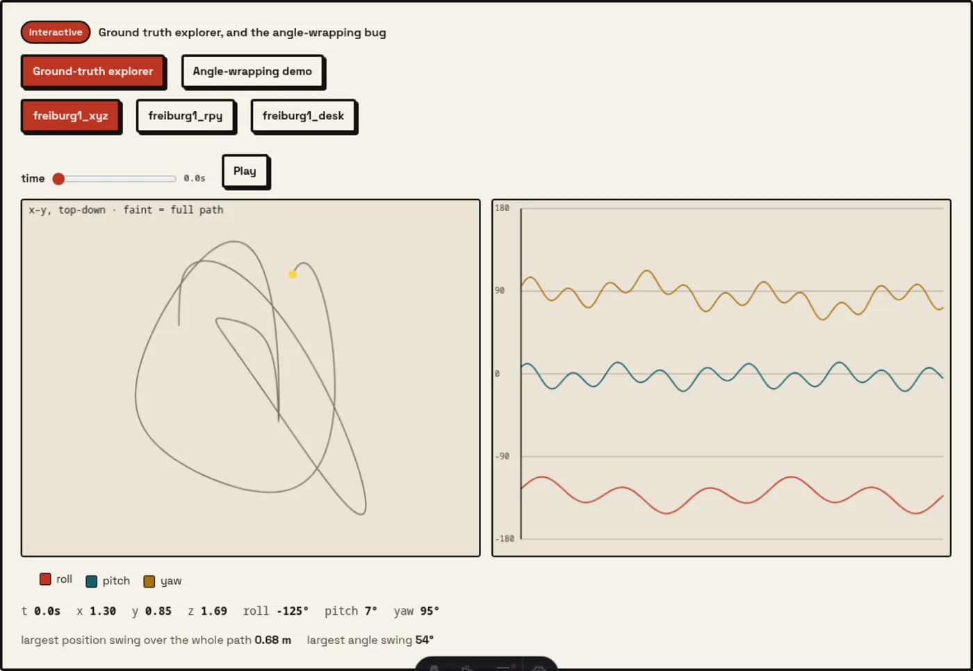
With JavaScript on: a time scrubber over synthetic xyz/rpy/desk paths with a synchronised orientation strip, and, switch the button above, a live demonstration of why naive angle subtraction breaks near ±180°.
Scrub the xyz sequence and the position trace does almost all the work while roll, pitch and yaw sit close to flat. Switch to rpy and the position trace barely leaves its box while the orientation strip swings through the full ±180° range, breaking cleanly at each wrap rather than drawing a spurious line through it, which brings us to a detail the report’s own figures get wrong.
Association, and the line everyone gets wrong
Once RGBD, ORB and EKF trajectories are all zeroed, createSummaryPlots.py lines 39–51
walks each system’s frames and finds the nearest ground-truth pose by timestamp:
for algName in Algs:
    trajdir = base_path + algName + "/" + datasetName + baseFileName
    X, Y, Z, roll, pitch, yaw, times, absTimes = getXYZABYTLists(trajdir)
    gtX, gtY, gtZ, gtroll, gtpitch, gtyaw, gttimes, gtAbsTimes = \
        getXYZABYTLists(ground_truth_dirs[datasetName], absTimes[0])
    eX, eY, eZ, eR, eP, eYaw = [],[],[],[],[],[]
    for i,atme in enumerate(absTimes):
        minTdiffi = np.argmin(np.abs(gtAbsTimes-atme))
        eX.append(X[i] - gtX[minTdiffi])
        eY.append(Y[i] - gtY[minTdiffi])
        eZ.append(Z[i] - gtZ[minTdiffi])
        eR.append((roll[i] - gtroll[minTdiffi]+180) % 360-180)
        eP.append((pitch[i] - gtpitch[minTdiffi]+180) % 360-180)
        eYaw.append((yaw[i] - gtyaw[minTdiffi]+180) % 360-180)
Position error is a plain subtraction, X[i] - gtX[minTdiffi], because metres don’t wrap.
Angles do, and line 49 is the fix: (roll[i] - gtroll[minTdiffi]+180) % 360-180. Without it,
a system reading 179° against a ground truth of −179° would report an error of 358° for what
is, physically, a 2° mistake. Every rotational number in this post depends on that one line.
Two RMSEs, and I can’t tell you which one is in the table
Lines 54–60, right after the association loop:
rmserror = np.sqrt((np.array(eX)**2+np.array(eY)**2+np.array(eZ)**2).mean()/3.0)
rot_rmserror = np.sqrt((np.array(eR)**2+np.array(eP)**2+np.array(eYaw)**2).mean()/3.0)
print(datasetName+algName+"   RMSE: "+str(rmserror*100))
print(algName+"   rRMSE: "+str(rot_rmserror))
rmserror = np.sqrt((np.array(eX) ** 2 + np.array(eY) ** 2 + np.array(eZ) ** 2).mean())
rot_rmserror = np.sqrt((np.array(eR) ** 2 + np.array(eP) ** 2 + np.array(eYaw) ** 2).mean())
print(algName + "   RMSE2: " + str(rmserror * 100))
The particle-filter report’s “RMSE” turned out to be a mean
squared error with no square root at all, a 960× headline that was really a 31× one. This
script isn’t that: both variables here do take a square root, so whichever one produced
Table 1 is at least a genuine RMSE. But there are two of them, and they don’t agree. The
first divides the summed squared per-axis errors by 3 inside the square root before
scaling to centimetres; the second doesn’t. That’s a factor of
apart, the difference between an average per-axis RMS and the combined 3-D displacement
RMSE that “positional RMSE” normally means in the SLAM literature. Nothing in the report
says which print line the numbers in Table 1 were copied from, and the run that produced
them isn’t reproducible without the ground-truth files either. I’ve quoted the table as
printed; take the absolute comparisons at face value and the exact centimetre figures with
a pinch of salt one way or the other.
The numbers
Read across xyz: 2.3 cm and 0.89° against two published systems at 0.86–1.7 cm and 0.43–0.52°. A hand-rolled EKF, built from Eq. (2.18) and a Jacobian assembled by hand, is within about a centimetre and half a degree of ORB-SLAM2 and RGB-D SLAM, on the sequence that’s mostly translation. Read across rpy: the positional gap barely widens (3.9 cm against 1.8–2.0 cm) but the rotational one explodes, 10.6° against 2.2–3.3°. Same filter, same tuning, one sequence where it’s nearly competitive and one where it is categorically worse, and the difference between those sequences is exactly the translation-vs-rotation split the widget above lets you feel.
Page 34, §6, gives the mechanism, and it’s the same one post 21 already found in the code: the observation Jacobian is a first-order Taylor expansion, valid near the linearisation point and nowhere else.
The EKF algorithm is inaccurate to largely rotational movements, as can be seen in the rotational RMSE values. This is due to the linear Taylor approximation performed on , as it assumes the function can be approximated with a linear function. Where this is true for small rotational movements, large rotational movements cannot be properly approximated and hence may not converge as expected.
Post 21 traced this to a specific commented-out line in the constructor (the report’s derived doesn’t match what shipped) and to the sub-block covariance update that never corrects an unobserved landmark. Neither of those is a rotation-specific bug; they explain why the filter is noisier everywhere. The rpy-specific failure is simpler and sits one level up: on a sequence built almost entirely from rotation, every correction starts further from where the linearisation is valid, so the same Jacobian is a worse approximation on every single frame.
Error against time
Figures 37–42 plot the same errors against time instead of collapsing them to one number.
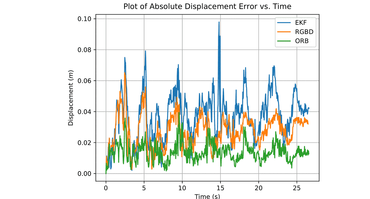
Figure 37, p.30. Positional error vs. time, xyz. EKF (blue) tracks RGBD (orange) and ORB (green) closely, with sharper peaks: never a different story, just a noisier one.
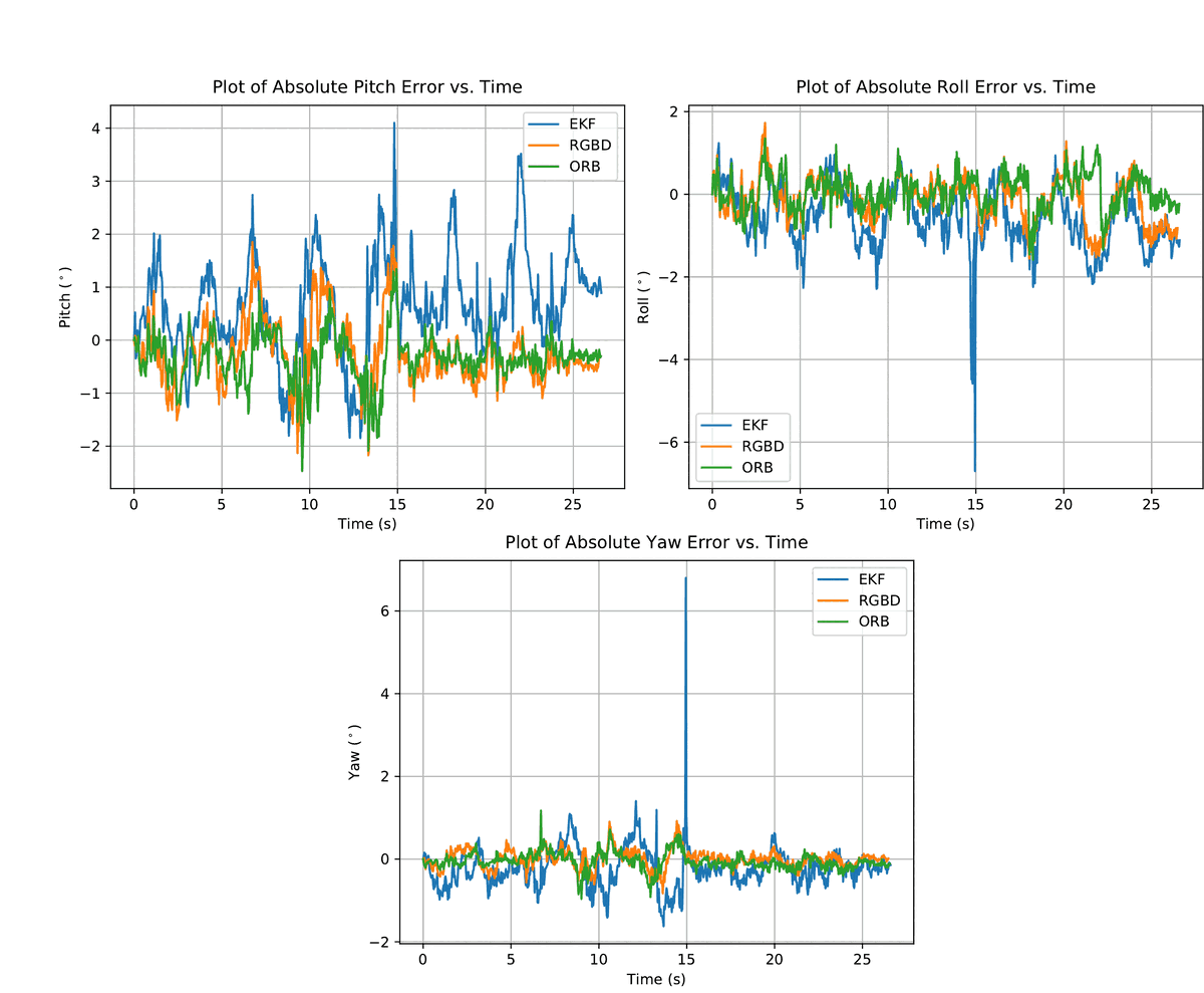
Figure 38, p.30. Rotational error vs. time, xyz. Watch the yaw panel around 15 seconds: a single-frame spike to nearly 7° that RGBD and ORB don’t share.
That yaw spike is a single bad correction, not a drift: it appears, and the very next points are back near zero. It’s the signature of exactly one frame whose observed landmarks were, briefly, matched with enough confidence to move the pose but not enough correctness to be right, the kind of frame the fix list below calls for RANSAC to catch before the filter ever sees it.
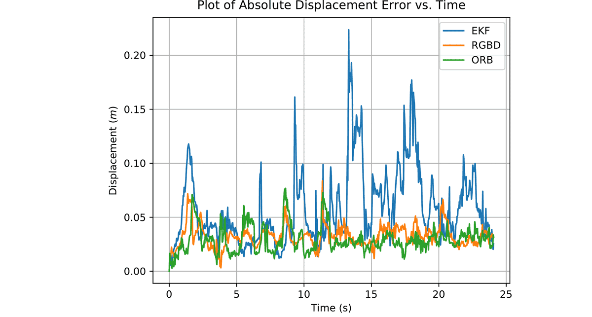
Figure 39, p.31. Positional error vs. time, rpy. Even here, where rotation dominates, the position error is still only around 2× RGBD’s and ORB’s, the real damage is elsewhere.
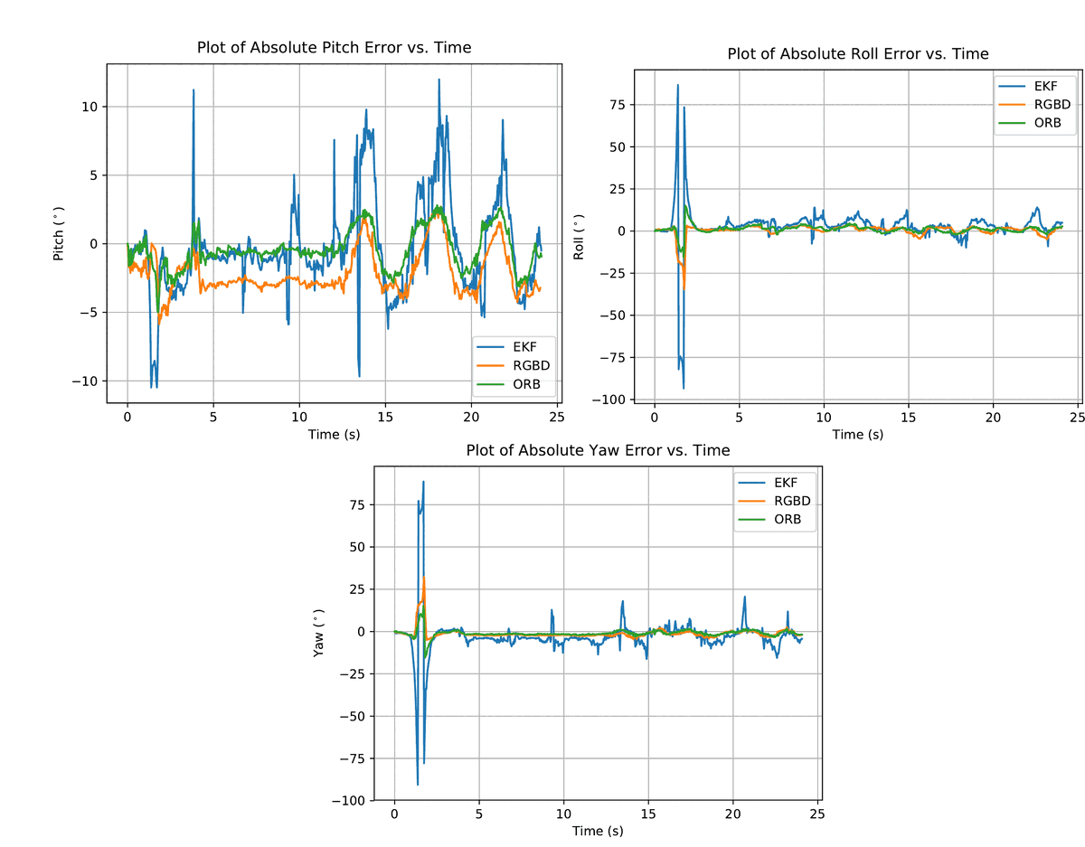
Figure 40, p.31. Rotational error vs. time, rpy, where the 10.6° in Table 2 actually lives. One burst near the start reaches almost 90° in both roll and yaw before settling; ten-degree excursions recur for the rest of the run.
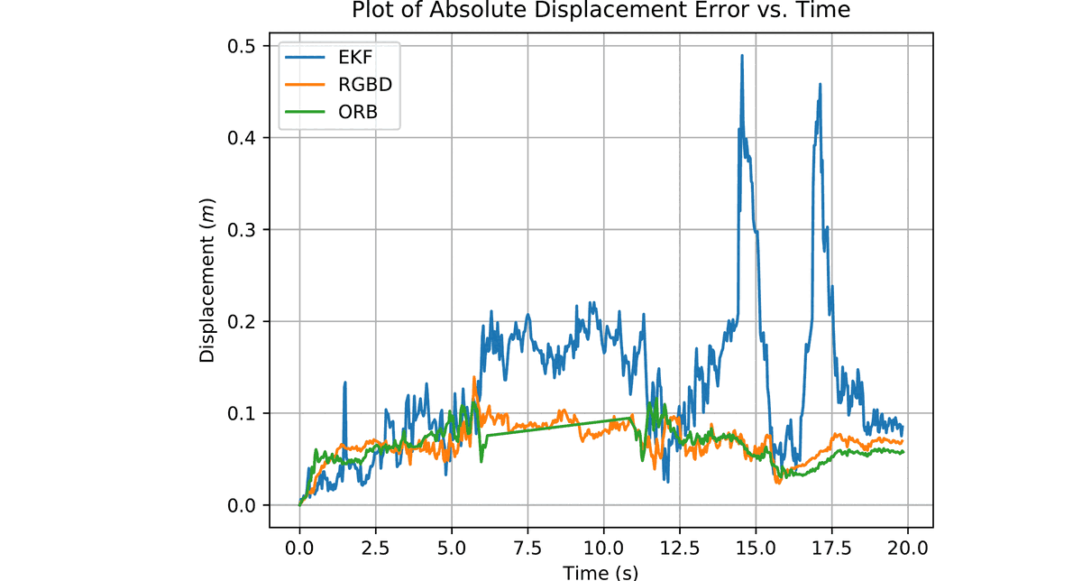
Figure 41, p.32. Positional error vs. time, desk. Look at the green ORB-SLAM2 line between roughly 5.7 s and 11 s, an unnaturally straight ramp, unlike every noisy segment either side of it.
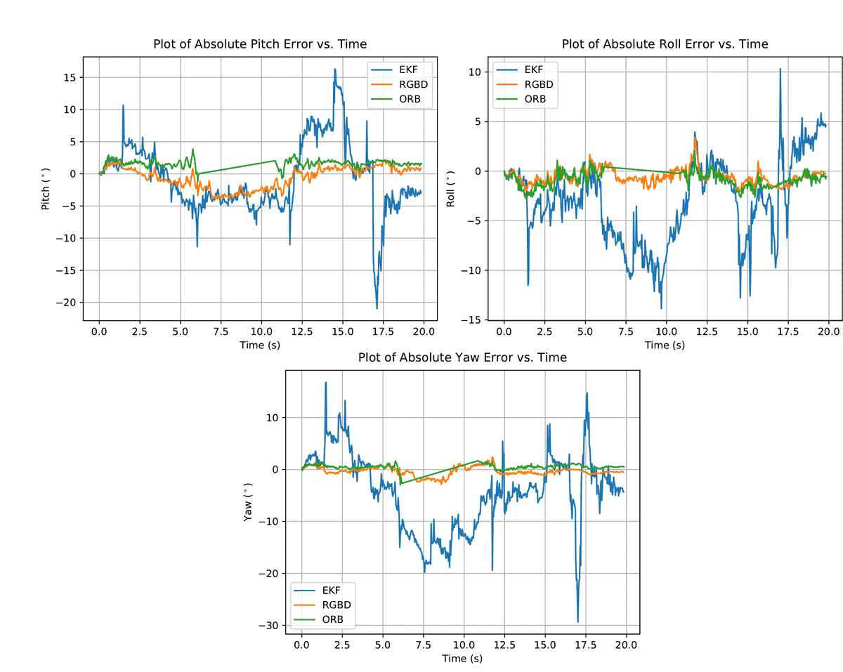
Figure 42, p.32. Rotational error vs. time, desk, the same straight segment shows up in all three of ORB’s channels, not just displacement.
That straight line is ORB-SLAM2 getting lost. Page 34: “on the desk dataset, the ORB SLAM
algorithm gets lost. This is due to a lack of features to track at one point in the motion.
However, it is able to recover very well. The artefacts of this can be seen in the summary
error graphs, where the ORB SLAM’s error is shown as a straight line for a short segment.”
While ORB-SLAM2 has no tracking estimate, createSummaryPlots.py still associates whatever
poses are logged to the nearest ground truth in time, and matplotlib draws a straight
segment across the gap between the last pose before tracking was lost and the first one
after relocalisation, an artefact of the plotting, not of the error itself, but a visible
signature of a real failure and recovery. It’s on all three rotational channels in Figure 42
as well as displacement in Figure 41, because the gap is in the pose stream, not in any one
axis.
What §6 would change
Page 34 is the densest page in the report: it compares the RGB-D SLAM numbers against a published baseline, explains the ORB-SLAM2 recovery above, diagnoses the EKF’s rotational weakness quoted earlier, and then lists four fixes, rephrased here with what I’d add now:
- Two descriptor sets, not one. Matching every frame against the whole map’s SURF descriptors is what makes relocalisation possible at all, but the set only grows, and a bigger set is a slower, noisier nearest-neighbour search. A recent set for tracking, with the global one as fallback when lost, is the fix, and it’s the same fix post 21’s own fix list reaches for.
- RANSAC on the correspondences, to catch the kind of single confidently-wrong match that produces the yaw spike in Figure 38, geometric rejection before the filter sees the measurement, rather than after the fact through a displacement gate.
- Loop closure and bundle adjustment, listed in the report as smoothing steps. Post 21’s read, with the code in front of it, is sharper: the loop closure the joint-covariance design is supposed to give for free was switched off by the matrix-extraction shortcut that also confines the update to the observed sub-block. Fix that first.
- A coarse motion estimate before the EKF, so the correction starts near the answer instead of at whatever the identity model predicts, and the first-order Jacobian is valid at the point it’s evaluated. This is the direct answer to the number in Table 2.
And, in the report’s own words, the honest alternative to all four:
An alternative Markov based approach, known as the Particle Filter (PF), would be more resilient to these effects. […] A motion model can also be applied to the PF-based algorithm. The PF based approach is compared to the EKF-based approach in Table 3.
That table hands the story back to where it started three months earlier: the particle filter posts, where the same EKF-vs-PF gap showed up as a 31× RMSE ratio on a bearings-only tracking problem, for the same underlying reason: a single Gaussian cannot sit on two modes at once, and a landmark that’s briefly ambiguous between two matches is exactly that.
Try the angle-wrapping bug yourself
Switch the widget above to Angle-wrapping demo. Drag heading a (what a system
measured) and heading b (ground truth) so they straddle the seam, the defaults already
do, at −175° and 170°, 15° apart in reality. The chart sweeps a across the full range with
b held fixed: the grey line is naive subtraction, unbounded and wrong the moment it leaves
the shaded ±180° band; the accent line is (a − b + 180) % 360 − 180, breaking cleanly at
the fold instead of running off the page. At the defaults, naive subtraction reports 345°
apart; the actual separation is 15°. That 23× error, silently averaged into an RMSE with
every well-behaved frame around it, is not a hypothetical: it is line 49 of
createSummaryPlots.py, and every rotational number in Tables 1, 2 and this post’s figures
depends on it having been written correctly.
What’s honest about this post
Everything in this post apart from the widget is transcribed from the report’s own text,
figures and code, with page and line references throughout. What isn’t reproducible: the three trajectory
files the tables and error plots were computed from, since Results/ was never committed,
so the figures are the report’s own matplotlib output, not this repo’s, and the “which RMSE
formula” question above is genuinely unresolved rather than dug out. What is fully live:
the ground-truth explorer (synthetic, clearly labelled so) and the angle-wrapping demo,
which needs no data at all and is, honestly, the most durable single fact in this post. I
have re-derived that % 360 gotcha from scratch in at least two other languages since 2018,
and gotten the sign wrong at least once more.