Blog · Research infrastructure ·
Four algorithms, one benchmark: what actually won
Four segmentation algorithms, one harness, the same ScanNet scenes: reconstruction error bounds everything, voxel size beats architecture, and the numbers do not say which one to actually ship.
- Interactive
- python
- semantic-segmentation
- 3d-reconstruction
- evaluation-metrics
- computer-vision
- research-infrastructure
This is the payoff post of a six-post series about the harness itself, not the algorithms it scored: the config that drove every run, the metrics that scored every prediction the same way, the greedy matcher behind the instance numbers, the geometry that let a point cloud be compared against image-space ground truth, the trajectory-error metrics, and the SWIG seam that made one of the four algorithms callable from Python at all. All of that exists so the numbers below are comparable in the first place. Four algorithms, the same ScanNet validation scenes, the same metric functions, the same pandas → LaTeX pipeline. This post is what the numbers say, what the renders show, and (because a benchmark table never says this part on its own) what they leave out.
The line-up
3DMV back-projects 2D CNN features from nearby posed images into a 3D voxel grid and
jointly predicts from the fused 2D+3D features: an offline method that needs a completed
mesh and a handful of colour images per voxel before it can say anything.
MinkowskiEngine, run here as MinkUNet34C, is a sparse 4D convolutional network over a
voxelised point cloud, also offline, and, as the harness ran it, run twice per scene at
two voxel sizes. SemanticFusion is the odd one out: a per-frame 2D CNN fused
incrementally onto a surfel map as the camera moves, the only one of the four that is
building its map while it predicts, and the only one with no completed mesh to fall back
on.
configs/run_algs_scannet_val.yaml is the exact config that produced every number below,
worth reading before the results, because it is also where the “run twice” detail lives:
# configs/run_algs_scannet_val.yaml:6-14
tests:
  - id: ExecuteAlg
    alg:
      id: MinkowskiEngine
      weights_path: "/data/algs/minkowski_runner/weights.pth"
    dataset:
      id: "SCANNET"
      file_map: "/data/datasets/scenenn_val_dataset.csv"
There is no voxel_sizes: key in that block. ExecuteMinkowskiEngineConfig defaults it:
# segtester/configs/alg/MinkowskiEngineConfig.py:9
self.voxel_sizes = BCNF.OptionalMember(default_ret=[0.05, 0.02])
and ExecuteMinkowskiEngine.__call__ loops over that list per scene, re-quantising the
same point cloud and re-running the same network at each size:
# segtester/algs/minkowski/minkowski.py:59-72
for voxel_size in tqdm(self.conf.voxel_sizes, desc="voxel_size"):
    ...
    sparce_tensor = generate_input_sparse_tensor(pcd, self.device, voxel_size)
So “MinkowskiEngine (2cm)” and “MinkowskiEngine (5cm)” in every table below are one config line, run twice, with everything else (architecture, weights, scene) held fixed. That is what makes the voxel-size finding below a controlled comparison rather than an apples-to-oranges one. 3DMV’s own voxel size is a separate, fixed hyperparameter three lines below it in the same config:
# configs/run_algs_scannet_val.yaml:15-23
  - id: ExecuteAlg
    alg:
      id: 3DMV
      model_path: "/mnt/1C562D12562CEDE8/MODELS/3DMV/scannetv2/scannet5_model.pth"
      model2d_orig_path: "/mnt/1C562D12562CEDE8/MODELS/3DMV/scannetv2/2d_scannet.pth"
      process_nth_frame: 5
      num_nearest_images: 4
      voxel_size: 0.048
4.8 cm, close to Minkowski’s 5 cm run, not its 2 cm one, which matters when you get to the per-class table. 3DMV’s 2D branch is a 41-class ENet trained on ScanNet’s own colour statistics:
# segtester/algs/mv3d/mv3d.py:28
ENET_TYPES = {'scannet': (41, [0.496342, 0.466664, 0.440796], [0.277856, 0.28623, 0.291129])}
and SemanticFusion’s config line that matters most for the “online” argument at the end of
this post is cnn_skip_frames:
# segtester/configs/alg/SemanticFusionConfig.py:9
self.cnn_skip_frames = BCNF.OptionalMember(default_ret=10)
That default, 10, means the CNN only re-predicts every 10th frame; every other frame, the surfel map is fused
from whatever the last CNN pass said (segtester/algs/semanticfusion/semanticfusion.py:119).
That is the mechanism, not just the number, behind SemanticFusion running live at all: it
does not pay the CNN’s cost on every frame.
Reconstruction error first, because it bounds everything else
Every one of the metrics below is scored against a reconstructed point cloud, not the ground-truth mesh, so before any semantic number means anything, it is worth asking how close that reconstruction is to the room it is describing.
| Algorithm | Mean [m] | STD [m] | Max mean error [m] | RMSE [m] |
|---|---|---|---|---|
| 3DMV | 0.016 | 0.009 | 0.018 | 0.018 |
| ME (2cm) | 0.011 | 0.006 | 0.013 | 0.013 |
| ME (5cm) | 0.026 | 0.016 | 0.029 | 0.031 |
| SemanticFusion | 0.095 | 0.152 | 0.766 | 0.201 |
The two offline voxel methods start from a mesh that was reconstructed once, off to the side, before either algorithm ever ran: 1.1–2.6 cm mean error, an order of magnitude tighter than SemanticFusion’s 9.5 cm mean and 20.1 cm RMSE, because SemanticFusion is building the mesh it predicts onto, frame by frame, while it tracks. The 0.766 m max-mean error is one scene having a bad day, and the RMSE is nearly triple the mean for exactly that reason: a handful of geometry-losing frames dominate a metric that squares its errors before averaging. Every semantic number in this post inherits that gap: SemanticFusion cannot possibly score well on a room it has not finished reconstructing yet.
Classification, instance, semantic: nine columns, one table
segtester/assessments/summarizeresults.py::SummarizeRes is the pandas → LaTeX pipeline
that produced every table in this post, including this one. create_seg_all_res_tex
(summarizeresults.py:273-289) pivots a results dataframe on alg_name, sums the raw
accuracy numerator/denominator across every scored scene rather than averaging
per-scene accuracies, and takes the mean of miou/fiou:
# segtester/assessments/summarizeresults.py:273-282
table = df.pivot_table(values=["miou", "fiou"], index=["alg_name"], aggfunc=np.nanmean)
t2 = df.pivot_table(values=["pt_acc_num", "pt_acc_den"], index=["alg_name"], aggfunc=np.nansum)
table.insert(0, 'Accuracy (%)', 100 * t2["pt_acc_num"] / t2["pt_acc_den"])
That numerator/denominator sum (not a per-scene mean) is why a big scene with lots of
points pulls accuracy toward itself more than a small one, a deliberate choice, and the
same “weight by how many points actually exist” idea FIoU applies per class
(Post 26 covers that formula in full; this post reuses
it, not re-derives it). “Classification” scores every point against the full class set;
“Instance” and “Semantic” both run the greedy instance matcher from
Post 27 first, with match_classes=True and False
respectively: the gap between those two columns is exactly the cost of getting the class
right and the extent right.
| Algorithm | Class. Acc. [%] | Class. FIoU | Class. MIoU | Inst. Acc. [%] | Inst. FIoU | Inst. MIoU | Sem. Acc. [%] | Sem. FIoU | Sem. MIoU |
|---|---|---|---|---|---|---|---|---|---|
| 3DMV | 57.316 | 0.459 | 0.373 | 48.034 | 0.392 | 0.044 | 40.815 | 0.340 | 0.032 |
| ME (2cm) | 73.592 | 0.695 | 0.681 | 54.407 | 0.448 | 0.214 | 50.831 | 0.419 | 0.175 |
| ME (5cm) | 54.922 | 0.442 | 0.288 | 38.349 | 0.276 | 0.085 | 31.551 | 0.219 | 0.044 |
| SemanticFusion | 34.325 | 0.207 | 0.161 | 26.036 | 0.208 | 0.010 | 20.942 | 0.160 | 0.007 |
Per class: where the coarse grid loses, and where it doesn’t
| Class | Acc 3DMV | Acc ME 2cm | Acc ME 5cm | Acc SF | IoU 3DMV | IoU ME 2cm | IoU ME 5cm | IoU SF |
|---|---|---|---|---|---|---|---|---|
| Bed | 58.121 | 95.188 | 30.597 | 25.744 | 0.089 | 0.310 | 0.102 | 0.039 |
| Books | - | - | - | 47.457 | - | - | - | 0.012 |
| Ceiling | - | - | - | 7.570 | - | - | - | 0.023 |
| Chair | 80.997 | 89.511 | 51.555 | 14.146 | 0.353 | 0.638 | 0.236 | 0.077 |
| Floor | 94.192 | 97.958 | 95.764 | 42.992 | 0.785 | 0.859 | 0.737 | 0.345 |
| Furniture | 59.140 | 86.057 | 32.747 | 28.317 | 0.261 | 0.591 | 0.151 | 0.132 |
| Objects | 4.510 | 9.855 | 0.138 | 22.690 | 0.046 | 0.094 | 0.002 | 0.109 |
| Picture | 15.990 | 72.211 | 1.259 | 14.115 | 0.054 | 0.358 | 0.011 | 0.027 |
| Sofa | 26.607 | 97.112 | 11.989 | 17.498 | 0.062 | 0.345 | 0.036 | 0.029 |
| TV | - | - | - | 0.048 | - | - | - | 0.000 |
| Table | 72.075 | 95.242 | 35.995 | 12.763 | 0.350 | 0.591 | 0.144 | 0.061 |
| Wall | 66.771 | 98.406 | 93.802 | 54.481 | 0.463 | 0.676 | 0.503 | 0.299 |
| Window | 67.983 | 90.788 | 47.803 | 16.464 | 0.155 | 0.552 | 0.209 | 0.059 |
Widen the lens and there’s a second, quieter deprivation-vs-detection story hiding in the
same columns. Picture (thin, flat, wall-mounted) drops from 3DMV’s 16.0% and ME (2cm)‘s
72.2% to ME (5cm)‘s 1.3%: a 5 cm voxel does not just miss small free-standing objects, it
erases thin surface detail too. Sofa tells the opposite story from Objects: ME (2cm)‘s
97.1% accuracy dwarfs SemanticFusion’s 17.5%, because a sofa is large and flat enough that a
fine voxel grid resolves it fine and an incrementally-built surfel map, mid-reconstruction,
frequently hasn’t finished it yet.
What the widget shows and what it can’t
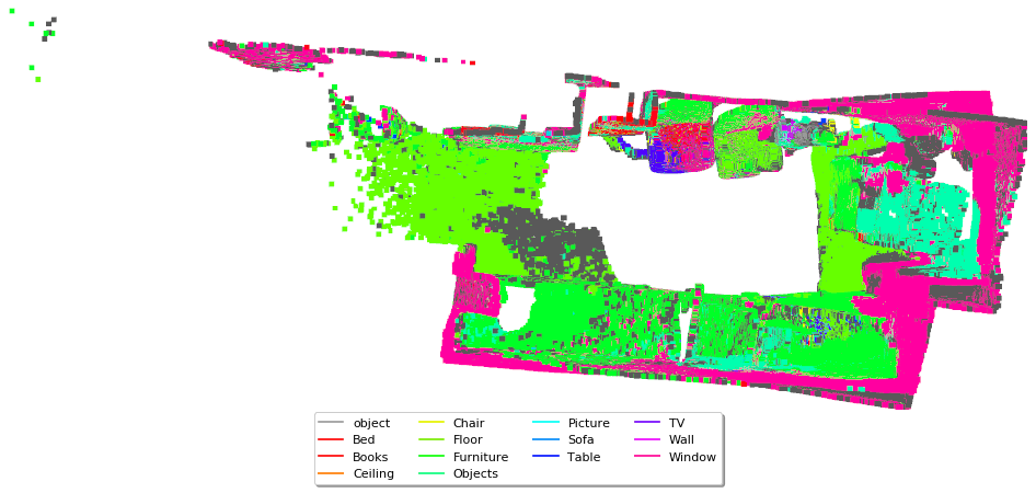
Static fallback: ground truth for scene0278_00, one of the three scenes the widget compares.
With JavaScript enabled, this becomes a scene picker (three ScanNet scenes with all four
renders committed), a 2×2 grid of ground truth / 3DMV / ME (2cm) / ME (5cm), a clickable
class legend that dims every panel to one class at a time, the results tables above as a
sortable table and metric-driven bar chart, a per-class small-multiples chart with
explicit gaps for the - classes, and four weighting sliders that reorder a live ranking
of the four algorithms.
The repo ships 16 renders in assets/SCANNET/common/: four scenes × (ground truth /
3DMV / ME 2cm / ME 5cm), but only three scenes have all four panels:
scene0278_00, scene0316_00, scene0423_00. scene0019_00 only has a ground-truth
render; scene0278_01 has all three algorithm renders but no ground truth. The widget uses
the three complete scenes and says so, rather than padding the picker with a panel that
would silently be missing.
Click Objects in the legend and the ME (5cm) panel goes almost entirely grey while SemanticFusion (not shown in these renders, since only the four ScanNet panels above are committed, but scored in every table on this page) is the algorithm the per-class table says handles it best. The renders make the voxel methods’ failure visible; they can’t make SemanticFusion’s relative strength visible in the same frame, because no SemanticFusion point-cloud render was ever committed to the repo. That’s a real gap in what’s available to show, not a decision to leave it out.
The reprojected 2D numbers, and the odometry number
SemanticFusion is the only algorithm run on NYUv2 as well as ScanNet, reprojected into 2D image space rather than scored in 3D, using the machinery Post 28 covers in full:
| SemanticFusion (NYUv2, 2D) | Accuracy [%] | FIoU | MIoU |
|---|---|---|---|
| Classification | 37.166 | 0.248 | 0.145 |
| Instance | 1.433 | 0.010 | 0.003 |
| Semantic | 21.471 | 0.182 | 0.045 |
SemanticFusion is also the only algorithm with an odometry number, because it’s the only one running its own SLAM tracking (ElasticFusion) rather than reading ground-truth poses:
What the numbers do not say
Nowhere in any table above is the one number that would change which algorithm a real
application should pick: SemanticFusion runs live, at roughly 10 Hz on a laptop GPU
(the number this repo’s README and the wider project report it at; no frame-rate benchmark
.tex table exists in this repo, so treat it as a stated figure, not a re-measured one).
3DMV and MinkowskiEngine do not run live at all: both need a completed mesh before they
can predict anything, which means an offline batch job, not a robot deciding what’s in
front of it right now. That’s not a footnote to the accuracy table; it’s a different axis
entirely, and it is completely invisible in every row above.
The widget’s weighting sliders are the point made operable: set “Frame rate” to its
maximum and everything else to zero, and SemanticFusion (dead last on every accuracy
column on this page) jumps to first. Set “Accuracy” and “mIoU” high and “Frame rate” to
zero, and ME (2cm) wins comfortably, same as the raw tables say. Neither ranking is wrong.
“Which algorithm is best” was never a well-posed question on its own; “which algorithm is
best for building a live map on a robot” and “which algorithm is best for offline,
maximum-accuracy scene labelling” are two different questions with two different
answers, both sitting in the same eight .tex files.
What I’d tell past me
Every one of the four numbers columns in this post’s headline table came out of the same
get_results function, the same SummarizeRes pipeline, scored on the same scenes. That’s
the entire point of building the harness first: Post 25’s
config-driven design, Post 26’s shared metric functions,
Post 27’s greedy matcher, Post 28’s
reprojection, none of which is interesting in isolation, and all of which is the only reason
a table with four algorithms in it means anything at all. The two findings worth remembering
past this specific benchmark: a hyperparameter you’d bury in a methods-section table
(voxel size) can matter more than the choice of architecture the paper’s title is about, and
a benchmark table has an axis it structurally cannot report (what a method costs to run)
that can flip the ranking entirely. Read the config before the leaderboard.