Blog · Stereo ·
z = bf/d: epipolar geometry and the simplest triangulation there is
Depth from two photographs, derived from nothing but two similar triangles: what assumptions buy that simplicity, why the result is a shape and not a measurement, and a playground where you drag a disparity by hand and watch the uncertainty wedge breathe.
- Interactive
- stereo
- epipolar-geometry
- triangulation
- 3d-reconstruction
The last three posts matched every pixel between two photographs and scored the result. This one asks a different question: once you have a match, one correspondence, however you found it, what do you actually get to say about the world? The dense posts never needed to answer that, because a disparity map is already the answer’s raw material. Sparse reconstruction is where it becomes explicit: pick a point in each image, and the report’s own §5 opening states the general method plainly.
“It is possible to reconstruct a 3d image from 2 views of a scene once one is able to identify correspondences in the image. This can be done by re-projecting the point from the reference image to a line in real-world coordinates using the inverse of the camera calibration matrix. This is then also done with the second image and the point of intersection between the two lines in the measured real-world co-ordinates of the point.”
That’s it, in general: back-project a pixel through the inverse of the camera matrix and you get a ray, not a point: a pixel only tells you a direction, not a distance. Do it again from the second camera and you get a second ray. Two rays through the same physical point generally meet, and the meeting point is the reconstruction. In practice, with real pixel noise, two rays almost never meet exactly: you’d take the midpoint of their closest approach, or solve it properly with a linear least-squares system (DLT), rather than trust an exact intersection that measurement error has already broken. None of that machinery appears in this repository, though, because the report immediately specialises to a much kinder case.
The rectified special case
Constrain the two cameras to differ by nothing but a horizontal shift (same orientation, same focal length, centres separated by a baseline along one axis) and the general back-project-and-intersect problem collapses to two similar triangles. This is Figure 16 of the report, redrawn below with the report’s own labels: camera centres , image planes at height , a world point , and its two projections .
Using similar triangles and , with the focal length and the world point’s horizontal offset from camera 1: . Using and : . Subtracting the first from a rearrangement of the second and solving for , with the disparity, gives the report’s Eq. 5.1:
That is the entire reconstruction. Multiply the baseline by the focal length, divide by however many pixels the point moved between the two images. Post 29 derived the same equation from the same two triangles for the dense case; here it is the whole of the algorithm rather than a motivating aside, because sparse reconstruction has no scanline sweep to speak of: once two points are known to correspond, is the only arithmetic left.
z ∝ 1/d, and what that costs you at range
Depth is inversely proportional to disparity, not linearly, and that one fact explains the shape of every stereo point cloud in this post. A point twice as far away moves half as far between the two images. Differentiate with respect to and you get the resolution directly: a one-pixel error in the match moves the recovered depth by
That’s quadratic in . The report notices the consequence without deriving it, in the §5.4 discussion of why FERN’s reconstructed points cluster the way they do:
“It is interesting to see that there are many regions close to the front of the image and fewer closer to the back. This is due to the fact that the distance is inversely related to disparity. Hence, points which have a low disparity are in the largely increasing portion of z, reducing the accuracy of those points.”
The widget’s depth-resolution panel is that sentence turned into a curve you can read a number off, rather than a shape you have to take on faith.
The code
Modules/D_Reconstruction.py is 32 lines, and it is the entire reconstruction step for
both matchers in this repo. The triangulation itself, D_Reconstruction.py:5-9:
def get3DFromDisparity(key_points, located_pts, img1, disparityscale, ground_truth_disparity=None):
    disparity = key_points[1]-located_pts[1]
    z = np.clip(1.0/(disparity+1e-10), 0, 0.2)
    colors = img1[np.rint(key_points[0]).astype(np.int32), np.rint(key_points[1]).astype(np.int32)]
    X = key_points/[[-img1.shape[0]], [img1.shape[1]]]
    X += [[0.5], [-0.5]]
Every matched keypoint pair produces one point: its disparity is a raw column difference, its colour is read straight out of the reference image at the keypoint location, and its plotting position is the pixel location rescaled into a plane (dividing by image height and width and recentring, the same normalisation the top-down schematic below sidesteps by working in real pixels throughout). Lines 13–18 build a comparison when ground truth is available:
    ground_truth_disparity = ground_truth_disparity/disparityscale
    z_real = np.clip(1.0/(ground_truth_disparity+1e-10), 0, 0.2)
    errors = ground_truth_disparity[np.rint(key_points[0]).astype(np.int32),
                                    np.rint(key_points[1]).astype(np.int32)]-disparity
    mesh = np.meshgrid(np.linspace(-0.5, 0.5, img1.shape[1]), np.linspace(0.5, -0.5, img1.shape[0]))
    return X, z, colors, mesh, z_real, errors
errors is a per-point disparity error, in pixels, and that’s what feeds the accuracy tables
in the FERN and SURF posts still to come. And the render, lines 21–31, does exactly two
things: scatter the coloured points, and lay a wireframe mesh of the ground-truth surface
underneath them:
def plot3DPoints(ax, X, z, colors, mesh=None, z_real=None):
    ax.scatter(X[1], X[0], z, c=colors, depthshade=False, marker='.')
    ax.set_xlabel('X Axis'); ax.set_ylabel('Y Axis'); ax.set_zlabel('Z Axis')
    if z_real is None or mesh is None:
        return
    ax.plot_wireframe(mesh[0], mesh[1], z_real, color=(0, 0, 0, 0.25), linewidth=1.0)
So every figure in §5.3 is a sparse, coloured point cloud floating over (or drifting away from) a faint grey surface it’s supposed to match. The widget’s top-down schematic borrows the same idea: the six channel markers’ true positions sit underneath the ray intersection as faint dots, so you can see how close a hand-picked disparity actually lands.
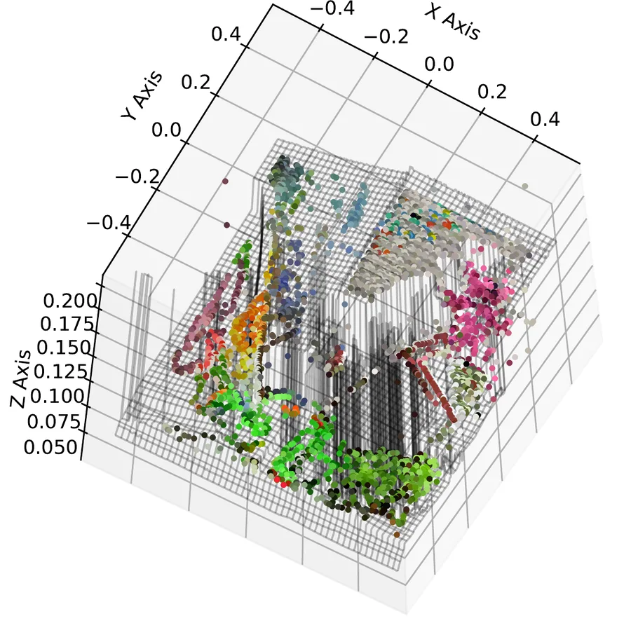
The repository’s own README banner (docs/pngs/results.png): the Cones scene,
reconstructed and coloured by plot3DPoints, sitting on its ground-truth wireframe.
The honest part: this is a shape, not a measurement
Look again at line 6: z = np.clip(1.0/(disparity+1e-10), 0, 0.2). There is no b and no
f anywhere in that line. bf has been set to 1.
The clip has a visible cost, and the widget’s projective mode reproduces it rather than
smoothing it over: with bf pinned at 1 and this repo’s usual disparities running from a
handful of pixels up past 30, sails past for almost every ordinary match, and
the clip flattens most of a scene onto one wall. It is only the very closest points
(biggest disparity, smallest ) that ever separate from that wall at all. Toggle to
metric, supply a real and , and the wall opens back out into six markers at six
different distances. That contrast is the whole point of §5’s caveat, made operable instead
of stated.
One more correction, while we’re here
The repository’s README.md opens with a claim the report itself contradicts:
“The FURN and SURF feature descriptors (from OpenCV) are used to match keypoints across multiple images.”
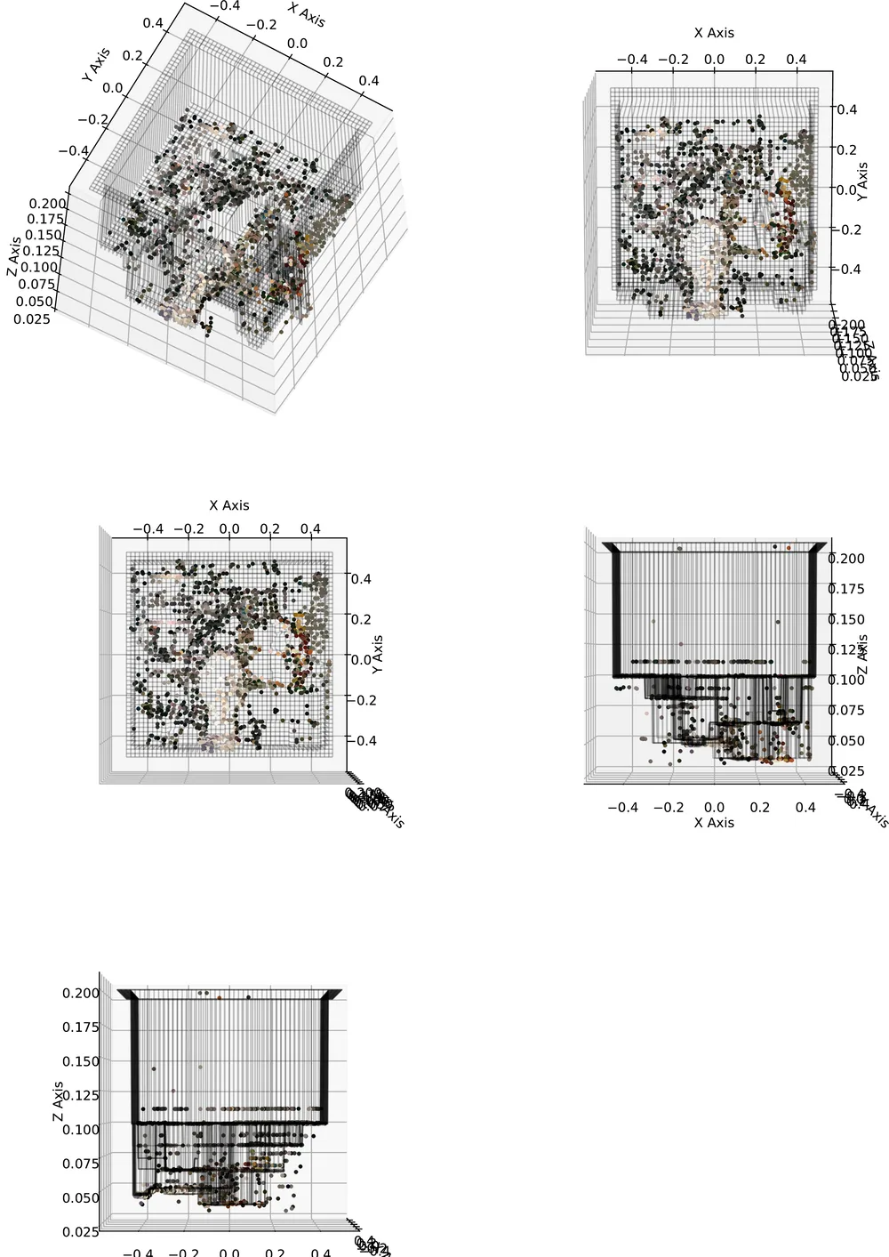
Figure 18: Tsukuba, FERN matcher, all five view_init angles the code produced.
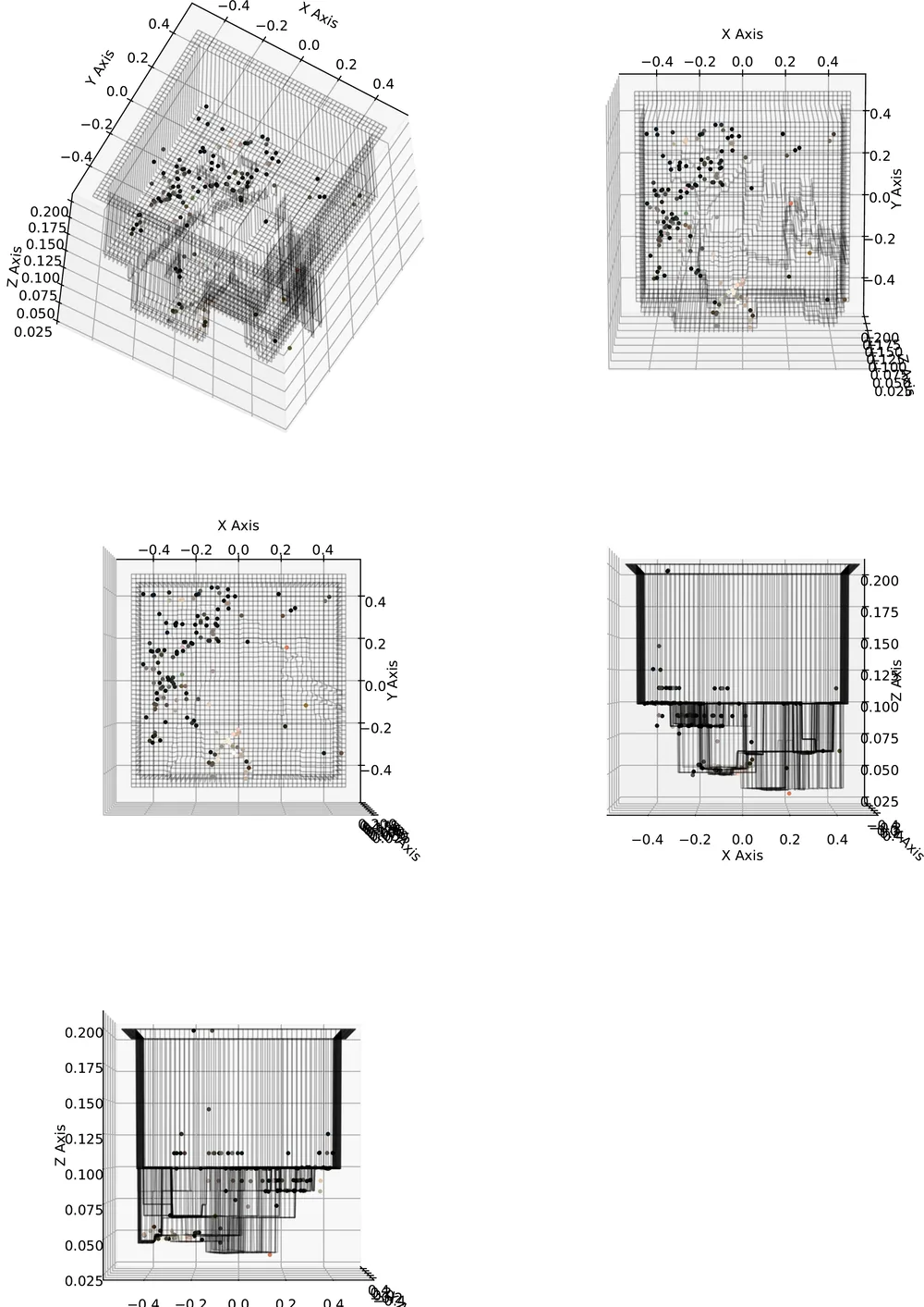
Figure 19: the same scene and the same five angles, SURF matcher. Visibly sparser.
FERN’s cloud is denser than SURF’s at every one of those five angles, a preview of the §5.4 trade-off (“FERN was able to correctly identify more points… however SURF had a higher accuracy rate”) that the FERN and SURF posts will take apart properly.
Try it: pick a disparity by hand
With JavaScript on, this becomes a synthetic stereo pair, six channel markers at known distances, six known colours, no photograph involved, where hovering the left image draws the live epipolar line in the right one, dragging a marker on that line picks a disparity by hand, and a top-down schematic redraws both camera rays, their intersection, and a shaded wedge showing how far that intersection moves for a ±1 px error. A depth-resolution curve turns z ∝ 1/d into a line you can read a number off, and a small reconstructed cloud replays the report’s own five viewing angles. A “verticalise the baseline” toggle rotates the second camera so the epipolar lines fan out to a finite epipole instead of staying horizontal: the one-click argument for why every scanline search in this series first assumes a rectified pair.
Four things worth doing with it.
Leave everything at its default and read the number. The scene was rendered with a 0.30 m baseline and a 360 px focal length; the metric sliders default to exactly that, so the marker starts on marker A’s true disparity and the schematic’s intersection lands on its true position, 4.0 m out. That’s the sanity check: the geometry is exact, so getting the inputs right gets the output right.
Now mis-set or and watch every point move together. The picture on screen doesn’t change (the pixel disparities are fixed, they came from the rendering camera, not from your sliders), but the interpretation of them does. A wrong focal length scales every recovered depth by the same wrong factor. That’s the projective-versus-metric distinction from a moment ago, made into something you break on purpose.
Drag the disparity down toward zero on a far marker and watch the uncertainty wedge open up. is quadratic in : at marker A’s 27 px disparity the wedge for a ±1 px error is a sliver; at marker F’s 2.7 px it swallows a large slice of the schematic. The depth-resolution curve underneath is the same fact with the scene-specific geometry stripped out: z ∝ 1/d as a curve, not a picture.
Tick “verticalise the baseline.” The right-hand image itself changes (camera 2 has yawed), and every epipolar line you can draw, at any hover position, now passes through one fixed point off to the side: the epipole. A horizontal-only scanline search, the kind dense stereo runs down every row, would be comparing pixels that have nothing to do with each other. This mode is a visual check only: the marker, the schematic and the depth readout switch off, because reading a real depth back out of a tilted pair honestly needs a fundamental matrix and a rectifying warp, and there is no rectification code anywhere in this repository to back that number up.
What’s next
The next two posts take the two matchers this one has been triangulating (FERN, feature
matching turned into a classification problem, and SURF, rebuilt from the paper with the
integral image I never got around to adding the first time around) through in full, using
the same z=bf/d from this post to put their points in space.