Blog · Features and preprocessing ·
Repeatability: benchmarking 12 feature detectors on the Oxford affine dataset
Detect, warp by a known homography, re-detect, count the hits: the repeatability metric, the fairness trick that makes it meaningful, and a ranking that completely reshuffles between zoom, blur, viewpoint, lighting and JPEG.
- Interactive
- feature-detection
- corner-detection
- repeatability
- fast
- harris
- shi-tomasi
- rust
- wasm
The previous post asked which edge detector survives noise. This one asks a version of the same question about corners (AGAST, AKAZE, BRISK, FAST, GFTT, Harris-Laplace, KAZE, MSER, ORB, SIFT, STAR, SURF, twelve of them) and the honest answer turns out to be a different question. “Which corner detector is best?” has no single answer. “Best under what transformation?” does, and the report has eight datasets and five image pairs each to answer it with.
Four ways to find a point worth keeping
Section 8 of the report (p. 32) sorts feature detectors into four families. Edge detectors (Sobel, the Laplacian, Canny, the subject of the last post) look for boundaries between regions, but edges are hard to track from one frame to the next, so they are rarely used for correspondence. Corner detectors, defined as the intersection of two edges, split further into three lineages the report names explicitly:
- Tree-based: AGAST, ORB, BRISK, all of them refinements of FAST (Rosten & Drummond, “Machine learning for high-speed corner detection”, 2006, reference [12] in the report’s bibliography, p. 51): a rule about the arrangement of pixels on a ring around a candidate point, extremely fast, but the least repeatable under scale and rotation.
- Difference-of-Gaussians: SIFT and SURF, slower, built on an image pyramid, generally more robust.
- Gradient-based: Harris-Laplace and GFTT (Shi-Tomasi), the eigenvalues of a local structure tensor, which is exactly the machinery this post’s widget builds.
- Unique: KAZE and AKAZE, which don’t fit the other three.
Blob detectors (MSER) and region-of-interest detectors round out the taxonomy but aren’t part of this experiment. Twelve detectors, four families, one question: put a transformation between two photographs of the same scene, and see which family’s points survive it.
What repeatability actually measures
Section 8.1.2 (p. 34) gives the protocol in seven steps, which I’ll paraphrase:
- Detect on image 1 of a dataset.
- Project those points into image N’s frame using the dataset’s known homography.
- Re-run the detector on image N.
- Count projected points that land within 3 px of an actual detection in image N.
- Count projected points that are still inside image N’s frame at all.
- Repeatability = step 4 ÷ step 5.
- Repeat for images 2 through 6, and for all eight datasets.
Step 5 matters more than it looks. A homography that zooms or rotates the scene pushes some
of image 1’s keypoints outside image N’s borders entirely. That’s not the detector’s
fault, it’s the crop’s, and punishing a detector for it would make wide-baseline datasets
look artificially bad. get_match_rate() in FeatureDetectionTesting.py (lines 7–22)
does exactly steps 2, 4 and 5:
def get_match_rate(kp_1_np, kp_2_np, T_1_2, img2_shape, thresh_sq):
    kp_T_1_2 = np.dot(T_1_2, kp_1_np.T)
    kp_T_1_2 = (kp_T_1_2 / kp_T_1_2[2]).T
    points_out_of_frame = np.count_nonzero(np.logical_or(kp_T_1_2[:, :2] >= img2_shape[:2],
                                                         kp_T_1_2[:, :2] < [0, 0]), axis=1)
    where_points_in_frame = np.where(points_out_of_frame == 0)
    kp_T_1_2 = kp_T_1_2[where_points_in_frame[0]]

    if len(kp_T_1_2)==0 or len(kp_2_np)==0:
        return float('inf')

    point_closer_than_thresh = np.sum(np.square(kp_2_np[:, None] -
                                                kp_T_1_2[None, :]), axis=2) < thresh_sq
    number_of_points_matched = np.count_nonzero(np.count_nonzero(point_closer_than_thresh, axis=0))
    match_rate = number_of_points_matched / len(kp_T_1_2)
return match_rate is the dataset’s homography and kp_1_np is every image-1 keypoint
in homogeneous coordinates, . The projection is the textbook one,
and the division by the third row on line 9 is that de-homogenisation. thresh_sq = 9 is
: the code compares squared distances so it never has to take a square root. Note
what get_match_rate is not doing: it is not matching a keypoint to its nearest neighbour
one-to-one. point_closer_than_thresh is a boolean grid (every image-2 keypoint against
every projected image-1 keypoint), and number_of_points_matched counts columns (projected
points) that have at least one image-2 keypoint within 3 px anywhere. Two projected
points that both land near the same real corner both count as matched. That is a slightly
generous definition of repeatability, and it is the report’s, not mine.
The fairness trick: fixing everyone’s keypoint count
If detector A returns 4,000 keypoints and detector B returns 400, A will look more “repeatable” by raw count almost regardless of quality, because it has more chances to land near something. Section 8.1.2 says the fix in one line: “the appropriate thresholds were adapted in order to keep a constant number of features between 350 and 500.” Every detector in this experiment is held to the same keypoint budget before it is allowed to compete.
The code that does the holding is detect_key_points() (FeatureDetectionTesting.py,
lines 63–97), and it’s a genuinely nice piece of engineering: a bisection-ish search that
brackets the target count without a derivative or a lookup table:
def detect_key_points(f, img, max_iterations=20, number_of_points_min=350, number_of_points_max=500):
    non_max = hasattr(f, "setNonmaxSuppression")
    if non_max:
        f.setNonmaxSuppression(True)
    kp = f.detect(img)
    if not hasattr(f, "getThreshold") or not hasattr(f, "setThreshold"):
        return kp, non_max, None
    current_step_positive_dir = None
    current_step_size = f.getThreshold()/10
    is_int_thresh = type(f.getThreshold()) == int
    for i in range(max_iterations):
        if len(kp) < number_of_points_min:
            if current_step_positive_dir:
                current_step_size = current_step_size/10
            new_thresh = f.getThreshold() - current_step_size
            if is_int_thresh:
                new_thresh = int(new_thresh)
                if f.getThreshold() == new_thresh:
                    break
            f.setThreshold(new_thresh)
            current_step_positive_dir = False
        elif len(kp) > number_of_points_max:
            if current_step_positive_dir == False:
                current_step_size = current_step_size/10
            new_thresh = f.getThreshold() + current_step_size
            if is_int_thresh:
                new_thresh = int(new_thresh)
                if f.getThreshold() == new_thresh:
                    break
            f.setThreshold(new_thresh)
            current_step_positive_dir = True
        else:
            break
        kp = f.detect(img)
    return kp, non_max, f.getThreshold()
Read it as: start with a step of one-tenth the current threshold. Too few keypoints? Lower the threshold by one step. Too many? Raise it. And the trick that makes it converge rather than hunt forever: every time the search reverses direction, the step shrinks by another factor of ten. The first few iterations can overshoot the band by a wide margin; each reversal narrows the bracket by 10×, so within twenty iterations the threshold has been walked down to within a fraction of a percent of wherever the 350–500 band actually sits for that image. It’s the same shape as bisection search, except the step size is inferred from the threshold’s own scale rather than from a known upper and lower bound, which matters here, because FAST and AGAST’s thresholds don’t share a scale with each other, let alone with Harris’s response value.
feature_detectors (further down the same file) hands detect_key_points() its starting
point per dataset: AGAST starts at threshold 40 on Bark, Graffiti and Leuven, 30 on Bikes,
60 on Boat and Trees, 50 on UBC and Wall; FAST starts at a flat 40 everywhere. The search
in the code above walks each of those starting points to wherever that particular image
needs it to land in the 350–500 band, once per image, before repeatability is ever measured.
Reading the tables
With JavaScript on, this becomes a sortable heatmap of Tables 1–8 (480 numbers): click a dataset to sort by it, a detector to trace its line across all eight, or a cell for its degradation curve.
Tables 1–8 (report pp. 37–40) are each a dataset: twelve detectors, five match rates (image
1 against images 2 through 6), and a dataset average. Transcribed once into data.json and
read as a heatmap rather than eight separate tables, the thing the plan promised is visible
in one glance: the ranking reshuffles, hard, and it reshuffles along the lines of what each
dataset actually varies.
| Dataset | Transformation | Winner (avg. %) | Runner-up (avg. %) |
|---|---|---|---|
| Bark | Zoom + rotation | BRISK (58.70) | SIFT (42.38) |
| Bikes | Blur | AKAZE (75.54) | ORB (73.30) |
| Boat | Zoom + rotation | BRISK (82.97) | ORB (72.69) |
| Graffiti | Viewpoint | BRISK (67.19) | ORB (56.17) |
| Leuven | Lighting | GFTT (75.45) | AGAST (60.87) |
| Trees | Blur | BRISK (51.48) | SURF (45.00) |
| UBC | JPEG compression | ORB (89.01) | Harris-Laplace (84.19) |
| Wall | Viewpoint | BRISK (73.84) | SIFT (59.03) |
BRISK tops all four of the zoom+rotation and viewpoint datasets (Bark, Boat, Graffiti and Wall), which is the strongest single pattern in the tables. Blur is the one place I’d correct the plan I started from: it isn’t a clean AKAZE/ORB sweep. AKAZE wins Bikes with ORB second, but on Trees it’s BRISK on top and ORB down in fourth (35.20%, behind SURF at 45.00% and SIFT at 40.62%): the same detector that dominates the geometric-transform datasets also takes one of the two blur datasets. GFTT’s win on Leuven and ORB’s on UBC are both clean: neither is challenged within ten points.
Harris-Laplace is the detector I expected to be uniformly bad, and the tables say something more specific than that:
| Dataset | Harris-Laplace avg. % | Rank (of 12) |
|---|---|---|
| Bark | 8.75 | 12th |
| Bikes | 19.60 | 12th |
| Boat | 9.72 | 12th |
| Graffiti | 11.02 | 12th |
| Leuven | 40.38 | 9th |
| Trees | 18.83 | 9th |
| UBC | 84.19 | 2nd |
| Wall | 15.57 | 12th |
Last on five of eight datasets, mid-table on the two it isn’t last or second on, and second place, beaten only by ORB, on UBC’s JPEG-compression sweep. A detector built around scale-space extrema of the Harris response turns out to have nothing to lose from JPEG blocking artefacts and quite a lot to lose from perspective distortion, which is a more interesting fact than “Harris-Laplace is bad” would have been.
The report’s own caution, from §8.3 (p. 48), discussing Table 16, the descriptor experiment’s worst-performing dataset, but true of Tables 1–8 as well:
Eight datasets, twelve detectors at their OpenCV defaults (bar the 350–500 tuning): enough to show that the ranking depends on the transformation, not enough to declare a universal winner. That’s the honest reading, and it’s also the whole thesis of this post.
Thirteen unpublished pages
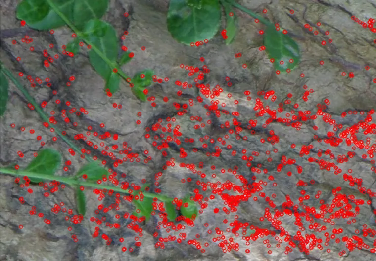
Appendix A (report pp. 52–64) draws every detector’s keypoints as red circles on all six
Bark images: thirteen pages, one detector per page (the thirteenth being the plain,
undetected source frame the code saves before the loop starts). The README embeds pages 1
through 51 and then wraps 52 through 98 in an HTML comment, so these renders have never
been on the public internet before. Below are three re-crops of that unpublished appendix:
BRISK, the zoom+rotation winner; FAST, the detector this post’s widget reimplements; and
Harris-Laplace, the detector that finishes last almost everywhere. All three are Bark image
1, cropped from report-png/report-54.png, report-55.png and report-57.png
respectively, page renders, not files from the dataset itself (see the note below the
widget further down).
BRISK on Bark, image 1 (Fig. 40, p. 54): the detector that wins four of eight datasets.
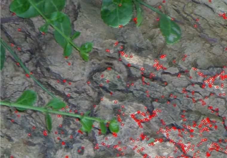
FAST on Bark, image 1 (Fig. 41, p. 55): the ~120-line detector below.
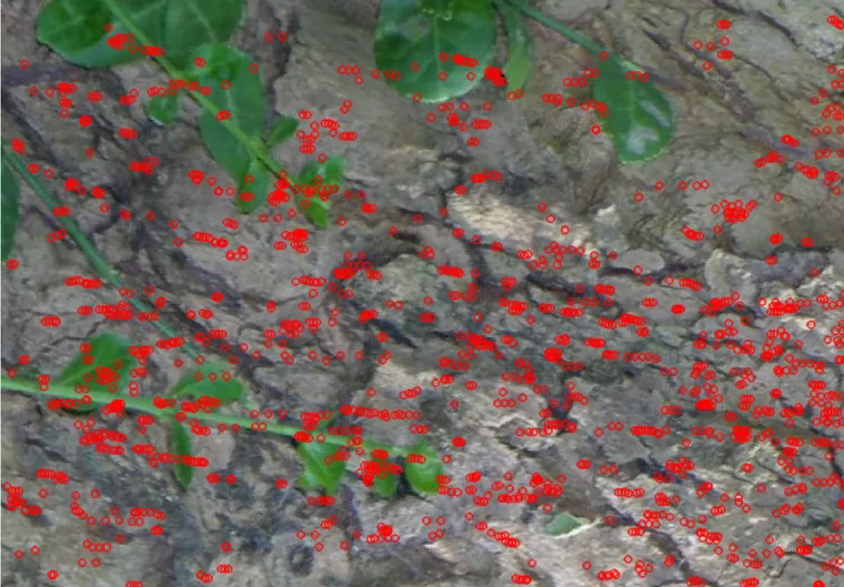
Harris-Laplace on Bark, image 1 (Fig. 43, p. 57): last on five of eight datasets, second on UBC.
FAST, Harris and Shi-Tomasi share a structure tensor
SIFT, SURF and BRISK are out of scope for the widget below: a DoG pyramid or a binary
descriptor pipeline is a much bigger build than this post’s crate budget, and Tables 1–8
above are where to go for how they actually compare. What the widget runs live are the three
detectors report §8 calls tree-based and gradient-based: FAST, Harris and Shi-Tomasi
(GFTT’s scoring function). All three live in a new module,
wasm/crates/imaging-wasm/src/corners.rs, added to the shared imaging-wasm crate this
site’s posts build on. lib.rs needed exactly one new line, pub mod corners;, to wire
it in; everything else, including every #[no_mangle] export, lives in the new file.
FAST: a 16-pixel ring and a contiguous-arc test
FAST asks one question at every pixel: does a run of at least consecutive pixels on a
16-pixel Bresenham ring around it (radius 3) all read brighter than the centre plus a
threshold, or all darker than the centre minus it? FAST_CIRCLE is the ring’s offsets in
scan order, and the contiguous-run test is the classic double-scan-of-32 trick for handling
a run that wraps past the array’s end:
fn max_circular_run(flags: &[bool; 16]) -> usize {
    if flags.iter().all(|&f| f) {
        return 16;
    }
    let (mut best, mut cur) = (0usize, 0usize);
    for i in 0..32 {
        if flags[i % 16] {
            cur += 1;
            best = best.max(cur);
        } else {
            cur = 0;
        }
    }
    best
}(corners.rs, lines 59–73.) fast_detect() (lines 80–118) builds the 16 ring values as
plain i32s (the whole test is integer arithmetic, exactly as Rosten & Drummond’s original),
checks the run length against (9 or 12, both selectable in the widget), and scores a
hit by summing how far past the threshold each of the 16 ring pixels reads in the winning
direction, which nms_local_max() (lines 123–150) then uses to keep only the local
maximum among a keypoint’s 8 neighbours. It is not OpenCV’s exact scoring function (OpenCV
bisections the threshold itself to find the largest one a pixel still passes), but it is
monotonic in “how much of a corner this is”, which is all non-maximum suppression needs.
Harris and Shi-Tomasi: two readings of one matrix
The report’s gradient-based family (Harris-Laplace and GFTT) both start from the same structure tensor,
built from one Sobel gradient and three windowed sums. Tensor::compute() (lines 192–208)
is the whole shared step:
pub fn compute(&mut self, gray: &[f32], window: usize) {
    let (w, h) = (self.w, self.h);
    sobel(gray, &mut self.gx, &mut self.gy, &mut self.tmp, w, h, 3, Border::Reflect101);
    for i in 0..w * h {
        self.ixx[i] = self.gx[i] * self.gx[i];
        self.iyy[i] = self.gy[i] * self.gy[i];
        self.ixy[i] = self.gx[i] * self.gy[i];
    }
    let k = window.max(1) | 1;
    box_running(&self.ixx, &mut self.sxx, &mut self.tmp, w, h, k, Border::Replicate);
    box_running(&self.iyy, &mut self.syy, &mut self.tmp, w, h, k, Border::Replicate);
    box_running(&self.ixy, &mut self.sxy, &mut self.tmp, w, h, k, Border::Replicate);
}
sobel is the same gradient the noise benchmark’s Canny uses
(edges.rs); box_running is Kernel Bench’s running-sum box
filter from rank.rs, reused rather than re-derived. Once Tensor holds sxx, syy
and sxy, Harris and Shi-Tomasi are both five-line functions of the same three numbers:
pub fn harris_response(t: &Tensor, k: f32, out: &mut [f32]) {
    for i in 0..t.w * t.h {
        let (a, b, c) = (t.sxx[i], t.sxy[i], t.syy[i]);
        let det = a * c - b * b;
        let trace = a + c;
        out[i] = det - k * trace * trace;
    }
}

pub fn shitomasi_response(t: &Tensor, out: &mut [f32]) {
    for i in 0..t.w * t.h {
        let (a, b, c) = (t.sxx[i], t.sxy[i], t.syy[i]);
        let trace = a + c;
        let diff = a - c;
        let disc = (diff * diff + 4.0 * b * b).max(0.0).sqrt();
        out[i] = 0.5 * (trace - disc);
    }
}
Harris’s response is (Harris & Stephens 1988); Shi
and Tomasi’s is the smaller eigenvalue of itself, . On a flat region both eigenvalues are near zero and both
responses read near zero. On a corner both eigenvalues are large, and a unit test
(harris_and_shitomasi_agree_on_a_corner_and_diverge_on_an_edge) checks that both readouts
call it a strong positive at a synthetic checkerboard crossing. On a straight edge, though,
they disagree in a way worth knowing about if you’re picking between them: one eigenvalue
is large and the other is (in principle) exactly zero, so Shi-Tomasi’s response floors at
zero (an edge is simply “not a corner”) while Harris’s term
makes an edge read strongly negative, a signed signal a thresholded Shi-Tomasi map
throws away. That’s the mechanism behind Harris’s optional response heatmap in the widget:
turn it on and the straight edges of whatever you point the camera at go visibly darker
than the flat regions around them, not just dimmer.
The auto-tuner, applied to two detectors that never had it
The report’s step-halving search only ever ran on FAST-shaped detectors: the
hasattr(f, "getThreshold") guard two sections up. Extending the same shape to Harris and
Shi-Tomasi is this post’s own idea, not a reproduction: autotune() (lines 288–321) is a
generic port of detect_key_points()’s loop that takes any count_at(threshold) -> usize
closure. Both Harris and Shi-Tomasi hand it a fraction of the frame’s own strongest
response rather than an absolute number: Harris’s response spans orders of magnitude
with image contrast, so a fixed threshold that works on one photo is either everything or
nothing on the next, and GFTT’s qualityLevel was already exactly this idea, which is
where Shi-Tomasi’s version of the control comes from. Toggle “hold count at 350–500” in the
widget below and watch whichever scalar that detector exposes get walked to a level that
lands there: the fairness trick from the tables, live on your own picture.
Corner Playground
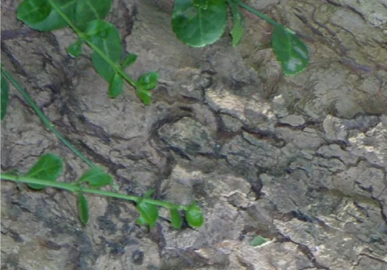
The widget’s bundled sample: Bark image 1 with no keypoints (report-png/report-58.png,
the plain frame the code saves before any detector runs).
With JavaScript on, this becomes a live FAST/Harris/Shi-Tomasi detector: pick the bundled bark crop, upload a picture, or use your camera, adjust each detector’s controls, and toggle the auto-tuner.
The camera is behind a button, freezes one frame rather than streaming continuously, and
degrades honestly: navigator.mediaDevices is undefined outside a secure context (plain
HTTP to a LAN address, notably how this site gets checked from a phone on the same
network), and the widget says so rather than looking like a silent permission failure.
Nothing you upload or photograph leaves your browser.
What I’d tune next
The widget’s Harris and Shi-Tomasi controls expose the same window that feeds
box_running for both: widen it and a real photograph’s corners get chunkier and fewer,
because the tensor is now averaging gradient products over a bigger neighbourhood. That’s a
free demonstration of something the report’s own experiment never varied: every table above
is one fixed set of OpenCV defaults per detector (bar the keypoint-count tuning), and §8.3’s
own caution, properly tweaking a detector to the problem can often greatly improve the
results, is a sentence the tables can’t act on but a slider can.