Blog · Regression ·
Automatic Relevance Determination: letting the model delete your useless features
Give a Gaussian process four input dimensions, two of them pure noise bolted on for the exercise, and a separate length scale per dimension is enough for it to work out which two matter on its own.
- Interactive
- gaussian-process
- ard
- kernel-methods
- regression
- rust
- wasm
The last post built the machinery: marginalise the basis away, and a Gaussian process is a prior over functions with four knobs: for magnitude, for how fast correlation decays with distance, and for a constant offset and a slope. It ended on a question. If can be learned by maximising the marginal likelihood rather than guessed, and you give every input dimension its own , the model can decide for itself which dimensions deserve a short length scale and which can be switched off. That is Automatic Relevance Determination, and this post is the assignment’s Part A doing exactly that to a four-dimensional problem where two of the dimensions are, by construction, garbage.
The mapping, and the two columns wired to nothing
Report §3.2 borrows a regression problem from MacKay: a 2-D robotic arm, Eq. (3.8),
with . Two hundred training points and two hundred test points: drawn from (a deliberate gap around zero), from , and Gaussian noise of variance added to the output. So far this is an ordinary 2-D regression problem. Then: “the variables and were chosen from a Gaussian distribution with a zero mean and a unit variance”, two more input columns, standard normal, correlated with nothing. never reads them. They exist purely so the fitting procedure has something to fail at ignoring.
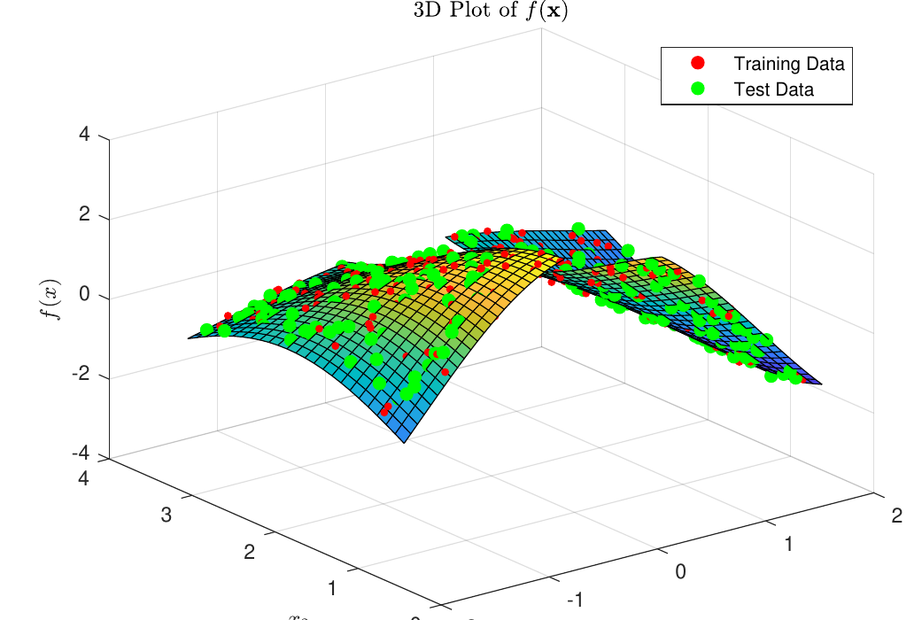
Report Fig. 6 (PDF p. 8, printed p. 6): the 3D plot of with training (red) and test (green) points. Only the top panel is shown here; the report’s three 2-D projections below it are not, since the widget’s own heatmaps below cover that ground interactively.
GP/data1_assignment3.mat ships , , , , the exact 200+200 draw
the report’s numbers come from. .mat files don’t run in a browser, so I exported the
four arrays to JSON with uv run --with scipy python -c "..." (scipy.io.loadmat,
never touching the source repo), into public/blog/automatic-relevance-determination/data/arm-data.json,
19 KB. That JSON is what the widget below trains on.
Two things before fitting anything
GP/PaQ2b.m lines 4-10 do two bits of preprocessing before the GP ever sees the data:
minX = min(X);
rangeX = max(X) - minX;
normX = (X - minX)./rangeX;
normXstar = (Xstar - minX)./rangeX;

meanY = mean(y);
yShifted = y-meanY;
Report Eq. (3.9) is the first three lines: every input dimension min-max normalised to using training statistics only, “to ensure that each variable has an equal prior weighting”. Without it, would start with roughly five times the raw scale of , and a single global would have to compromise between them, and the entire reason ARD needs a length scale per dimension would be half-defeated by leaving the dimensions on different footings before the model even starts. Eq. (3.10) is the last two lines: the targets get their mean subtracted, so the zero-mean GP assumption from the last post holds. The widget does the same, using only the training set’s own min/max/mean, never the test statistics, which is the point.
The kernel, and an erratum the report doesn’t know it has
Report Eq. (3.7), the ARD variant of the kernel, with a separate per input dimension inside the exponent:
GP/PaQ2b.m’s actual covfunc is {'covSum', {'covSEard','covNoise'}}: no ,
no , just the squared-exponential ARD term plus a noise term. So the kernel this
post is actually about is the first term alone, and everything below implements that.
Read as printed, multiplies directly, a precision. A large should mean the kernel decorrelates fast along axis : two points a hair’s breadth apart in that dimension become uncorrelated, which sounds like the opposite of “irrelevant”. And that is exactly what the report’s own discussion on p. 12 seems to say: “this causes the correlation to decrease rapidly for small changes in , which means that and will have a negligible effect on ”, reasoning from a large value to a fast decay to negligible effect, in that order.
But covSEard is GPML’s, and GPML’s documentation is explicit about what its
hyperparameters are: hyp.cov = [log(ell_1), .., log(ell_D), log(sf)], log length
scales, entering the kernel as , not .
GP/FormatData.py line 10 does np.exp(hyp.cov) and the result is what Table 1 below
calls , so the table’s is really , the length scale, and the two
readings give opposite meanings to “large”. Under a precision, large means sensitive;
under a length scale, large means the axis is so unimportant its exponent term never
moves the kernel regardless of how far apart two points are along it.
Only the length-scale reading survives contact with the report’s own results. A precision
of on would send to machine-zero for every pair
of training points that don’t happen to share a value on that axis, which, being
continuous, is every pair, collapsing the whole covariance to a near-diagonal matrix and
the model to noise. Table 2’s NRMSE of about 1% rules that out. A length scale of
does the opposite: stays negligible for any realistic difference,
so the term the report wanted to vanish, vanishes. I built wasm/crates/gp-wasm’s kernel
the length-scale way, ,
and reproduced Table 1’s numbers to three figures (below). The report’s own conclusion,
” and don’t matter”, is right; the mechanism its p. 12 paragraph gives for why
has the direction backwards, in the same spirit as the Eq. (3.7) typo the last post
found, a second small, genuine error in the same
equation’s neighbourhood, and a fun one to catch on a second pass.
Fitting it: five restarts, one basin
GP/PaQ2b.m’s optimisation, report Fig. 7 (PDF p. 9):
meanfunc = [];
covfunc = {'covSum', {'covSEard','covNoise'}};
likfunc = @likGauss;

besthyp = 0;
besthypScore = inf;
for c = 1:5
  hyp = struct('mean', [], 'cov', log(rand(1,6)), 'lik', -1);
  [hyp2, fX, iterations] = minimize(hyp, @gp, -2000, @infGaussLik,
      meanfunc, covfunc, likfunc, normX, yShifted);
  if fX(end) < besthypScore
    besthyp = hyp2;
    besthypScore = fX(end);
  end
end
Six random hyperparameters per restart, four length scales, , and covNoise’s
own noise term, drawn as , so every of them starts in
; hyp.lik (the likelihood’s own noise, a separate term from covNoise’s) is
fixed at every time, not randomised. minimize runs conjugate-gradient descent on the
negative log marginal likelihood for up to 2000 function evaluations, and PaQ2.m’s
predictions and errors (Fig. 8, PDF p. 10) are a direct port of Bishop’s mean/variance
formulae from the last post.
Report Table 1 (PDF p. 10), 10 independent restarts, transcribed:
| Run | Cost | |||||||
|---|---|---|---|---|---|---|---|---|
| 1 | 4.71e-01 | 7.68e-01 | 1.52e+04 | 75.58 | 2.50 | 6.92e-03 | 5.08e-02 | −2.513e+02 |
| 2 | 4.71e-01 | 7.68e-01 | 1.79e+04 | 75.59 | 2.50 | 9.91e-03 | 5.03e-02 | −2.513e+02 |
| 3 | 4.71e-01 | 7.68e-01 | 1.15e+04 | 75.59 | 2.50 | 5.47e-04 | 5.12e-02 | −2.513e+02 |
| 4 | 4.71e-01 | 7.68e-01 | 9.09e+03 | 75.58 | 2.50 | 5.06e-02 | 8.31e-03 | −2.513e+02 |
| 5 | 4.71e-01 | 7.68e-01 | 3.78e+04 | 75.59 | 2.50 | 3.25e-05 | 5.12e-02 | −2.513e+02 |
| 6 | 4.71e-01 | 7.68e-01 | 1.18e+04 | 75.59 | 2.50 | 3.64e-02 | 3.61e-02 | −2.513e+02 |
| 7 | 4.71e-01 | 7.68e-01 | 1.50e+04 | 75.58 | 2.50 | 2.43e-02 | 4.51e-02 | −2.513e+02 |
| 8 | 4.71e-01 | 7.68e-01 | 1.01e+04 | 75.58 | 2.50 | 5.09e-02 | 5.50e-03 | −2.513e+02 |
| 9 | 4.71e-01 | 7.68e-01 | 1.38e+04 | 75.59 | 2.50 | 5.12e-02 | 2.92e-03 | −2.513e+02 |
| 10 | 4.71e-01 | 7.68e-01 | 1.63e+04 | 75.58 | 2.50 | 5.49e-03 | 5.09e-02 | −2.513e+02 |
(Table 1 also lists each run’s initial hyperparameters; I’ve dropped that half. Every
initial is exactly , confirming hyp.lik=-1 really is fixed rather
than randomised, and the initial / values are just ten unremarkable draws
from .)
Table 2, the resulting errors:
| Training | Testing | |
|---|---|---|
| MSE (%) | 0.23 | 0.25 |
| RMSE (%) | 4.82 | 4.98 |
| NRMSE (%) | 0.97 | 1.06 |
What ARD actually found
Report p. 12, rephrased, one of the two best paragraphs in the write-up:
converges to about and to about 75.5, both large next to and . Ten independent restarts land on essentially the same values, so this is a real optimum, not a fluke of one random seed. And converges near , so , the true noise variance the data was generated with, which the optimiser was never told.
Read as length scales, this is a clean story. and get short length scales, 0.47 and 0.77, on inputs normalised to , meaningfully short relative to the domain, so nearby points really do correlate and the GP can interpolate between them. and get length scales in the tens of thousands and the tens: on a input, a length scale of 75 already makes negligible for any pair of training points, and makes it more negligible still. The exponent’s sum over four terms is dominated entirely by the two that matter. And the noise recovery is the part I’d call the actual payoff of the exercise: nothing in the optimisation objective mentions 0.0025, or MacKay’s arm, or that two of the four columns are meaningless, yet the same marginal-likelihood maximisation that killed also landed within a few percent of the true noise variance, purely because a Gaussian likelihood’s marginal is the one place where “explain the data” and “estimate how noisy the data is” are the same computation.
How many points does a robotic arm need? Ask Nyquist.
Report §3.3 swaps in a harder mapping, Eq. (3.14):
Ten times the frequency in . Before fitting anything, the report asks a question regression writeups almost never ask: how many training points does this actually need? Not “as many as I can afford”, a number, derived. The move (p. 13, Eq. 3.15) is to treat as a signal and invoke the Nyquist sampling theorem, which says the sampling rate must be at least twice the signal’s highest frequency component. The highest frequency term in is , angular frequency ; in it is ‘s own term, . Apply Nyquist per dimension and multiply, over each dimension’s actual sampled range:
Then, deliberately: “In order to ensure that enough points are generated for regression,
is multiplied by a factor of 8”, no derivation given for the 8, just stated as a
safety margin, landing on roughly 65 training points. GP/PaQ2d.m line 15 hardcodes
Ntraining = 65, matching rounded up. The safety factor is the honest
part: Nyquist gives the theoretical minimum for exact reconstruction of a
band-limited signal from noiseless samples on a regular grid; this sampling is random, not
a grid, the training points are 2-D not 1-D-per-axis, and a GP is not doing Shannon
reconstruction, it is doing Bayesian regression with a smoothness prior. None of that
makes the rigorous, but it is a real, numbered acknowledgement that the
bare-minimum count is almost certainly too few, which is a more disciplined way to pick a
sample budget than most regression writeups bother with.
GP/PaQ2d.m lines 15-20 draws the actual points, noiseless this time, and
dropped entirely:
Ntraining = 65;

X = [((1.932-0.45)*rand(Ntraining,1)+0.45).*(randi([0,1],Ntraining,1)*2-1) ...
    (3.142-0.534)*rand(Ntraining,1)+0.534];

y = 2*cos(10*X(:,1)) + 1.3*cos(sum(X,2));The harder mapping: same optimiser, two answers
GP/PaQ2dP2.m reruns the Fig. 7 procedure on the new data: 10 restarts, hyp.cov = log(rand(1,4)) (two length scales, , covNoise, since now), hyp.lik = log(10e-10), i.e. , fixed. Report Table 3 (PDF p. 11), transcribed:
| Run | Cost | |||||
|---|---|---|---|---|---|---|
| 1 | 1.61e-01 | 5.11e-01 | 1.04 | 1.35e+00 | 1.00e-09 | 1.188e+02 |
| 2 | 1.61e-01 | 5.11e-01 | 1.04 | 1.35e+00 | 1.00e-09 | 1.188e+02 |
| 3 | 7.36e-02 | 1.33e+00 | 4.73 | 6.69e-04 | 1.00e-09 | −1.210e+01 |
| 4 | 2.95e-01 | 1.13e-02 | 1.09 | 1.25e+00 | 1.00e-09 | 1.233e+02 |
| 5 | 7.36e-02 | 1.33e+00 | 4.72 | 6.68e-04 | 1.00e-09 | −1.210e+01 |
| 6 | 7.36e-02 | 1.33e+00 | 4.72 | 6.68e-04 | 1.00e-09 | −1.210e+01 |
| 7 | 1.61e-01 | 5.11e-01 | 1.04 | 1.35e+00 | 1.00e-09 | 1.188e+02 |
| 8 | 7.36e-02 | 1.33e+00 | 4.73 | 6.69e-04 | 1.00e-09 | −1.210e+01 |
| 9 | 7.36e-02 | 1.33e+00 | 4.72 | 6.67e-04 | 1.00e-09 | −1.210e+01 |
| 10 | 1.61e-01 | 5.11e-01 | 1.04 | 1.35e+00 | 1.00e-09 | 1.188e+02 |
Table 3 splits cleanly into two clusters, unlike Table 1’s single one: six restarts land at cost with –0.30, four land at cost with and , a genuinely lower (better, since this is a minimised negative log likelihood) cost, reached from a minority of starting points. Table 4:
| Training | Testing | |
|---|---|---|
| MSE (%) | 0.4205 | |
| RMSE (%) | 6.4844 | |
| NRMSE (%) | 0.9998 |
Report p. 16, rephrased, the second of the two best paragraphs:
The search space here is more complex: it takes more iterations to reach low cost, both because there are fewer training points and because the function itself is harder. Of the converged hyperparameters, is far smaller than : the output is more correlated with (which the term makes vary ten times faster) than with . collapsing to a tiny value is consistent with there being no noise in this data at all, reflected in the training NRMSE, negligibly small. Unlike §3.2, the confidence interval increases toward the centre of the input range, because the function changes faster there and the GP has to react to faster than the training points can pin it down.
The crate
This is the strongest linear-algebra case across both repos: one likelihood evaluation is
a Cholesky of a covariance, and a gradient step needs the gradient of the
log marginal likelihood with respect to all six hyperparameters. Analytic ARD gradients
are fiddly, a trace of per hyperparameter, on top of
the Cholesky itself, so wasm/crates/gp-wasm takes the fallback the plan calls out as
legitimate: a forward-difference gradient, one extra Cholesky per hyperparameter. For
the arm dataset’s six hyperparameters that is Choleskys of per
gradient step, times up to 20 backtracking line-search retries in the worst case, times 50
steps a button press: the “visible freeze in JS, well under a second in WASM” the plan
predicted. Timing it, one log_marginal_likelihood call is a fraction of a millisecond in
WASM, so even a worst-case press stays comfortably interactive.
gp-wasm is small and self-contained (not calib-wasm, whose SVD belongs to the camera
posts): wasm_alloc/wasm_free copied verbatim from example-wasm, and a gp_new/
gp_free opaque-handle pair (the pattern segment-wasm’s em_new/em_free uses) so
training data crosses the WASM boundary once and every other call, a slider move, an
optimiser step, is cheap integers, floats and pointers. The kernel, Cholesky, log
marginal likelihood, the finite-difference gradient-ascent optimiser (with backtracking,
so the likelihood is non-decreasing by construction, not an accident of a well-behaved
surface) and the predictive mean/variance are in wasm/crates/gp-wasm/src/gp.rs, pure
safe Rust over slices; lib.rs is only the unsafe pointer plumbing. cargo test -p gp-wasm has four cases: the log marginal likelihood against a hand-computed
case (independent 2×2 algebra, not sharing code with the Cholesky under test); the
Cholesky factor reconstructing the original matrix and its solve reproducing a direct
matrix inverse (); the optimiser’s recorded trajectory never decreasing over 30
steps; and a length scale on a deliberately-irrelevant synthetic dimension growing to more
than five times the real dimension’s after 60 steps. All four pass. pnpm build:wasm gp-wasm produces a 19.6 kB .wasm, comfortably inside the ~200 kB budget, most of
it the tests it doesn’t ship.
Numbers, honestly compared
I ran gp-wasm’s own optimiser on the exported arm dataset, 10 restarts,
log(rand()) inits exactly as PaQ2b.m does, 2000 gradient steps (matching the report’s
iteration budget, not the widget’s default 50), before trusting the kernel convention
above. The best restart landed at (the report’s cost column is
, so is the same number to three figures) with ,
, , noise , matching Table 1 to two or three
significant figures on every one of those. came out at 6.2 against the report’s
2.50, and reached 323 rather than the report’s –. Both
differences have the same explanation: gp-wasm carries one noise term where the report’s
covNoise+likGauss combination has two (the simplification Table 1’s own
non-identifiability justifies, above), which shifts how much of the “explain this away”
work has to do alone; and ‘s likelihood gradient is, by the time
is already in the hundreds, so close to zero that a forward-difference estimate
with a fixed step can’t reliably detect further improvement. The model has already
concluded is irrelevant in every way that matters (the exponent term is already
of the kernel’s dynamic range), it just doesn’t keep marching the number out to
five figures the way 2000 evaluations of a smoother analytic gradient does. Press “run the
optimiser” in the widget below a few times and you can watch keep creeping
rightward on the bar chart for exactly this reason, in ever-smaller steps.
The harder mapping’s multi-modality was harder to reproduce than I expected. Across 40
restarts at a generous 500-step budget, gp-wasm’s optimiser converges to the same
basin on my regenerated 65-point set every time, no second cluster like Table 3’s. But at
the widget’s realistic 50-step-per-press budget, the picture changes: one restart out of
15 landed at (badly overfit-to-noise-that-isn’t-there, tiny
, large noise) against for the rest. That is a real practical
multi-modal failure mode, just not necessarily a permanent second optimum in my
simplified model, more likely a slow-escaping bad region that a longer run eventually
leaves. Either way, “the restart you start from decides the answer” holds at the step
budget anyone actually presses a button for, which is the honest version of what the
report’s Table 3 shows.
Try it: ARD explorer
The heatmap on the left is the predictive mean over the plane (the frozen convention from report Figs. 9-11: where those dimensions exist), training points overlaid; the one on the right is the predictive standard deviation, same axes, same points. Four log-length-scale sliders, only the first two active on the harder mapping, which has no junk dimensions to switch off, plus and noise, and a live log marginal likelihood readout underneath.
Things worth doing, in order:
- On the arm dataset, drag (or ) upward from 1. Watch the mean heatmap: nothing changes. That axis was already frozen at for the plot, so its length scale can’t visibly affect this view; what it changes is how much the training points along that hidden axis are allowed to disagree with each other without being penalised, which is exactly the effect the log marginal likelihood readout tracks even when the picture doesn’t.
- Drag down toward 0.1. The mean surface goes from a smooth ridge to a speckled mess pinned tightly to each training point and flat everywhere else, a length scale too short to generalise between them, and the heatmap lights up almost everywhere off the training points.
- Press “run the optimiser”. Fifty real gradient-ascent steps, animated: the sliders sweep to where the optimiser actually walked, not a straight-line tween, and the bar chart at the bottom updates live: settle short, keep growing. That growing-without-bound bar is the argument, as a picture.
- Switch to “harder mapping” and press “restart from random” a few times. Each press
draws fresh hyperparameters and immediately re-optimises, the way
PaQ2dP2.m’s loop does. Watch the final log marginal likelihood: it doesn’t always land in the same place. - Under reduced motion, the optimiser still runs the full 50 steps, it just applies the result in one jump rather than animating the sliders through it.
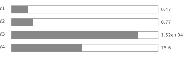
With JavaScript on this becomes a live ARD fit against the real 200-point arm dataset (or a regenerated 65-point harder mapping): two predictive heatmaps, six sliders, a “run the optimiser” button that animates 50 real gradient-ascent steps computed in WebAssembly, and a “restart from random” button for hunting a second optimum. The static picture is the report’s own converged values, as a bar chart, the shape the widget’s optimiser converges toward on the arm dataset.
What ARD buys, and what it costs
Nothing here changed the model class: it’s still one squared-exponential kernel, same as the last post. What changed is that the model now has one length scale per input dimension instead of one for all of them, which turns “is this input relevant” from a modelling decision made in advance into a number read off after fitting. That is a genuinely different kind of feature selection from choosing a subset of columns beforehand: it costs extra hyperparameters and, per this crate, extra Choleskys a gradient step, and in exchange it does not need you to have been right about which columns to drop before you saw the data. The harder mapping’s Table 3 is the honest asterisk on all of it: the same machine that reliably finds a single answer on one problem finds two, restart-dependent, on another, and the log marginal likelihood genuinely does not know which one you wanted.